Forest inventories often revisit only part of their plots in a given year. We extend the spatial model so nearby plots can share information both across space and across measurement years. The magnitude effect and the species factor now vary with location and time. We estimate their covariance parameters, map combined intercepts, and compare forest species-by-DBH densities at the beginning and end of the study.
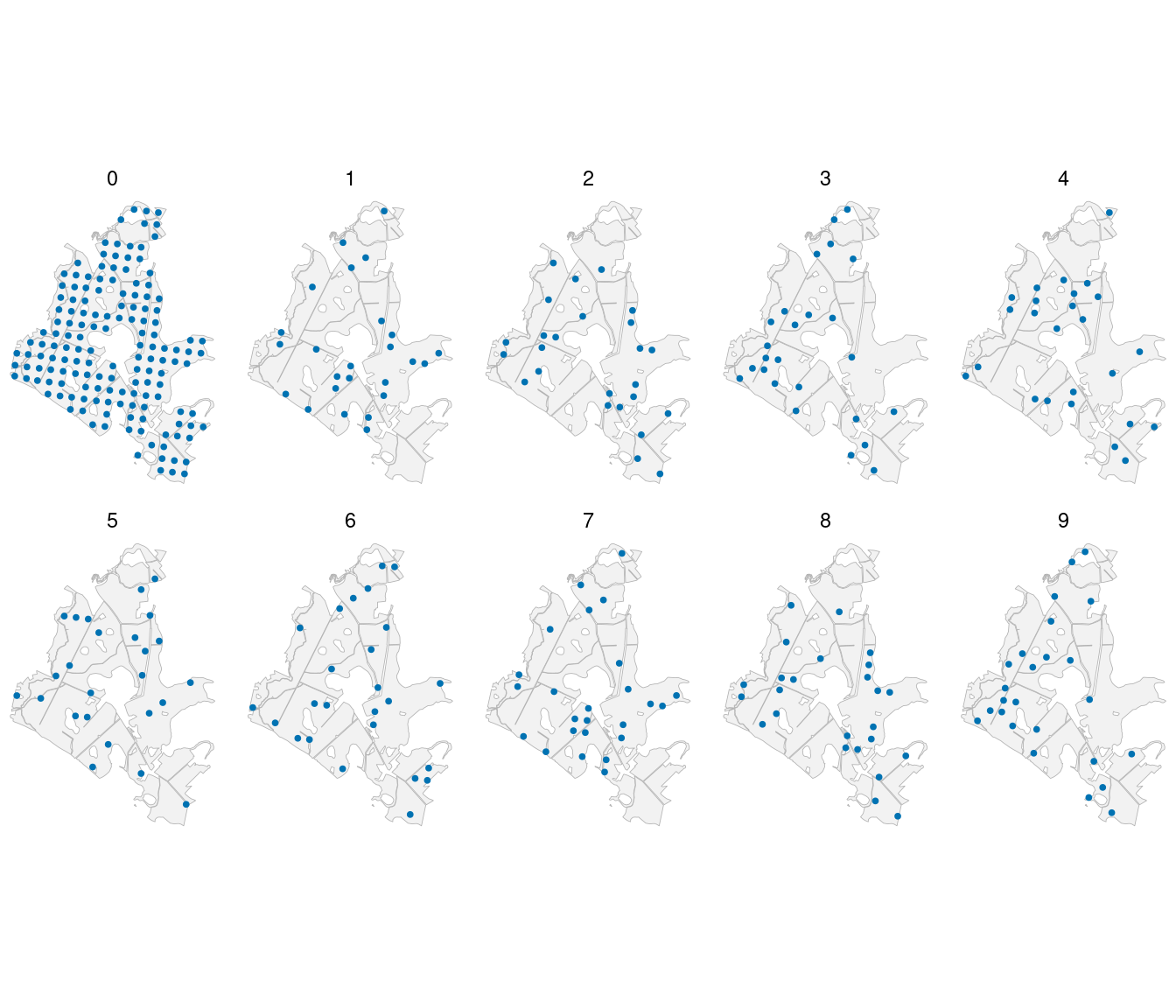
The example starts with all 151 plots in year 0 and revisits 25 plots in each of years 1 through 9, giving 376 plot measurements. It uses the same forest geometry and LiDAR canopy heights as the data article (Spitta et al. 2026). Counts are simulated. Canopy height is held constant over time so changes in this example arise through the space-time effects.
Example data
Download the space-time data (ZIP)
Extract the archive and use the folder containing data/ as your R working directory. It includes the generated counts, known effects, forest polygons, and generate_population.R. Reading these files avoids generating the full GP population again; the optional generator uses seed 1.
Read the repeated measurements
site_id identifies a physical location. plot_id identifies a measurement at a particular site and year, so repeated measurements have different plot_id values. The prediction file contains the 4,812 forest cells in years 0 and 9. location_id links each prediction to its cell polygon.
| 0 |
151 |
| 1 |
25 |
| 2 |
25 |
| 3 |
25 |
| 4 |
25 |
| 5 |
25 |
| 6 |
25 |
| 7 |
25 |
| 8 |
25 |
| 9 |
25 |
We map the measurements to see how the inventory covers the forest over time.
plot_locations <- plots |>
  st_as_sf(coords = c("easting", "northing"), crs = st_crs(forest), remove = FALSE)

ggplot() +
  geom_sf(data = forest, fill = "grey95", color = "grey70", linewidth = 0.15) +
  geom_sf(data = plot_locations, color = "#0072B2", size = 0.7) +
  facet_wrap(~ year, ncol = 5) +
  coord_sf(datum = NA) +
  theme_void()
Describe the space-time model
The magnitude model retains the same regression and negative-binomial count likelihood, with a space-time effect in the log density,
Here is standardized canopy height, is area in hectares, and is measurement year. The separable exponential covariance is
The spatial decay governs dependence with distance, and the temporal decay governs dependence with elapsed time. Larger values give faster decreases in correlation. At a fixed site, latent effects a year apart have correlation . At a fixed year, the model reduces to the exponential spatial covariance used in the spatial-effects article.
Species allocation uses an independent, unit-variance space-time factor,
with correlation . The loadings describe species responses to this common factor; is its temporal decay. Pine is the positive anchor, oak has its own loading, and birch receives the remaining trees. DBH allocation within species uses the same canopy-height regressions as the full-model article, without additional random effects.
We generate the magnitude field with , , and , and the species field with and . Spatial distances are in kilometers and time differences are in years. Magnitude coefficients are and ; size is . Pine and oak loadings are 0.7 and -0.5.
Optional full-GP population generation
The supplied script first selects the measurement schedule and sets the parameters. Each site appears at most once in each year.
library(tidyverse)

locations <- read_csv("data/locations.csv")
years <- 0:9

set.seed(1)

# All 151 sites are observed initially. Revisit 25 sites in each later year.
plot_sites <- locations |> filter(dataset == "plot") |> pull(site_id)
visit_order <- sample(plot_sites)
visits <- bind_rows(
  tibble(site_id = plot_sites, year = 0),
  expand_grid(year = 1:9, visit = 1:25) |>
    mutate(site_id = visit_order[((year - 1) * 25 + visit - 1) %% 151 + 1]) |>
    select(site_id, year)
)
beta_0 <- log(350)
beta_1 <- -0.2
sigma_v <- 0.5
phi_v <- 3
lambda_v <- 0.35
phi_w <- 5
lambda_w <- 0.25
size <- 1000
alpha_pine <- c(intercept = 0, slope = 0.5)
alpha_oak <- c(intercept = -0.5, slope = -0.5)
loading_pine <- 0.7
loading_oak <- -0.5
Separability lets us generate the full GP with a spatial Cholesky factor and a temporal Cholesky factor. If contains independent standard Normal values, has the required covariance across sites and years. Both the observations and prediction cells are included in these draws. The spatial matrix still requires more memory than reading the supplied data.
# One matrix draw contains every spatial location in every year.
# Rows index sites; columns index years. For a separable covariance,
# L_space %*% Z %*% t(L_time) is an exact full-GP draw.
distance <- as.matrix(dist(select(locations, easting_km, northing_km)))
time_lag <- abs(outer(years, years, "-"))

L_space <- t(chol(exp(-phi_v * distance)))
L_time <- t(chol(exp(-lambda_v * time_lag)))
Z <- matrix(rnorm(nrow(locations) * length(years)), nrow(locations))
v <- sigma_v * L_space %*% Z %*% t(L_time)

L_space <- t(chol(exp(-phi_w * distance)))
L_time <- t(chol(exp(-lambda_w * time_lag)))
Z <- matrix(rnorm(nrow(locations) * length(years)), nrow(locations))
w <- L_space %*% Z %*% t(L_time)
rm(distance, L_space, L_time, Z)

# Keep the sampled visits and the forest grid at the first and last years.
new_sites <- locations |> filter(dataset == "prediction") |> pull(site_id)
support <- bind_rows(visits, expand_grid(site_id = new_sites, year = c(0, 9)))
locations <- support |>
  left_join(locations, by = "site_id") |>
  mutate(plot_id = row_number(),
         v = v[cbind(site_id, year + 1)],
         w = w[cbind(site_id, year + 1)])
The rest of generate_population.R draws negative-binomial totals, allocates them to species and DBH classes, and writes the CSV files. Run source("generate_population.R") to reproduce the population.
Fit the model
We arrange the counts into one row per measurement, species, and DBH class. Time belongs to the measurement, so every category row for a given plot_id has the same year and coordinates.
species_order <- c("pine", "oak", "birch")
dbh_classes <- c("10-20", "20-30", "30-40", "40-50", "50+")

trees <- plots |>
  select(plot_id, area, x, easting_km, northing_km, year, contains(":")) |>
  pivot_longer(contains(":"), names_to = c("species", "dbh_class"),
               names_sep = ":", values_to = "count") |>
  mutate(species = factor(species, levels = species_order),
         dbh_class = ordered(dbh_class, levels = dbh_classes))

dat <- magCompData(trees, unit = plot_id, categories = c(species, dbh_class),
  tree_count = count, ordered = c(species = FALSE, dbh_class = TRUE),
  design = fixedArea(area))
The final coordinate in a space-time term is time. cov_model = "sep_exp" selects the separable exponential correlation. We use 15 neighbors and set st_scale = 0.25, making a one-year gap equivalent to 0.25 km when selecting neighbors. This search scale stays fixed; the covariance uses the actual spatial and temporal differences and estimates their separate decays.
The package supplies automatic priors and starting values. Here we explicitly set uniform supports for the decays to show how to specify them. The same supports apply to the magnitude field and the species factor, whose parameter values are estimated separately.
covariance_prior <- list(phi = uniform(0.3, 10), lambda = uniform(0.05, 1))

fit <- magComp(
  dat,
  magnitude = ~ x + nngp(easting_km, northing_km, year, cov_model = "sep_exp",
                          st_scale = 0.25, m = 15, name = "space_time"),
  composition = magCompComposition(
    species ~ x + factor_nngp(easting_km, northing_km, year,
      cov_model = "sep_exp", st_scale = 0.25, m = 15,
      anchors = "pine", name = "space_time"),
    dbh_class | species ~ x
  ),
  priors = magCompPriors(
    magnitude = list(terms = list(space_time = list(covariance = covariance_prior))),
    composition = list(blocks = list(species = list(
      terms = list(space_time = list(covariance = covariance_prior)))))
  ),
  control = magCompControl(n_samples = 8000, n_burn = 3000, n_chains = 3,
    n_cores = 3, chain_seeds = 1:3, nb_size = 1000, verbose = FALSE)
)
Each chain retains 5,000 draws. Size remains fixed because the magnitude model includes a random effect. magCompCovModels() lists the other available covariance families. magCompSettings(fit) reports resolved priors, starting values, and tuning. A covariance parameter can be held fixed with fixed(value) in its corresponding starting entry.
Examine parameters and combined intercepts
We compare the magnitude and species parameter estimates with their known values. The temporal decays appear as lambda_v and lambda_w[pine]; the loading rows have parameter = "loadings".
parameter_summary <- summary(fit)

parameter_comparison <- parameter_summary |>
  filter(component == "magnitude" | block == "species") |>
  left_join(true_parameters, by = c("component", "block", "parameter", "index"))

parameter_comparison |>
  select(symbol, truth, mean, q2_5, q97_5, rhat, ess) |>
  knitr::kable(digits = 3,
    col.names = c("Parameter", "Truth", "Mean", "2.5%", "97.5%", "R-hat", "ESS"))
| beta[0] |
5.858 |
5.803 |
5.687 |
5.956 |
1.062 |
53.547 |
| beta[x] |
-0.200 |
-0.227 |
-0.277 |
-0.175 |
1.001 |
175.220 |
| sigma_v^2 |
0.250 |
0.261 |
0.209 |
0.332 |
1.004 |
810.742 |
| phi_v |
3.000 |
3.413 |
2.352 |
4.673 |
1.004 |
561.436 |
| lambda_v |
0.350 |
0.439 |
0.260 |
0.703 |
1.001 |
933.747 |
| alpha[0,pine] |
0.000 |
-0.082 |
-0.323 |
0.081 |
1.012 |
69.541 |
| alpha[x,pine] |
0.500 |
0.574 |
0.498 |
0.651 |
1.006 |
250.198 |
| alpha[0,oak] |
-0.500 |
-0.467 |
-0.583 |
-0.300 |
1.015 |
74.643 |
| alpha[x,oak] |
-0.500 |
-0.551 |
-0.614 |
-0.492 |
1.013 |
289.151 |
| lambda[pine,pine] |
0.700 |
0.686 |
0.617 |
0.769 |
1.000 |
181.783 |
| lambda[oak,pine] |
-0.500 |
-0.487 |
-0.555 |
-0.429 |
1.002 |
252.734 |
| phi_w[pine] |
5.000 |
5.145 |
3.518 |
7.034 |
1.002 |
403.373 |
| lambda_w[pine] |
0.250 |
0.265 |
0.158 |
0.432 |
1.003 |
636.704 |
The intervals for both spatial and temporal decays include their generating values, as do those for the magnitude variance and species loadings. The magnitude intercept has a larger R-hat, about 1.06. Intercepts and latent effects can trade off while leaving their sums nearly unchanged. As in the spatial article, we also inspect the combined intercepts, averaged over the measured plot visits within each posterior draw.
summary(fit, type = "combined", group = ".all") |>
  select(component, stick, mean, rhat, ess) |>
  knitr::kable(digits = 3)
| magnitude |
|
5.816 |
1.000 |
1578.759 |
| composition |
pine |
-0.082 |
1.000 |
3170.132 |
| composition |
oak |
-0.467 |
1.006 |
2281.609 |
The combined-intercept R-hats are close to one, with much larger effective sample sizes than the separate intercepts. These diagnostics concern the combined coefficients. They do not replace checking the separate covariance and loading parameters in the preceding table.
Predict the forest in two years
We supply all cells in both years in one prediction call, retaining their joint space-time dependence. The observation target draws new counts and allocations in addition to new latent effects. We use 50 draws per chain for the figures and summaries, while keeping every fitting draw for diagnostics.
set.seed(1)

predictions <- predict(
  fit,
  prediction |> select(plot_id, area, x, easting_km, northing_km, year),
  type = "density", target = "observation", summary = "samples",
  n_draws = 50, keep_effects = TRUE
)
Map true and estimated relationships
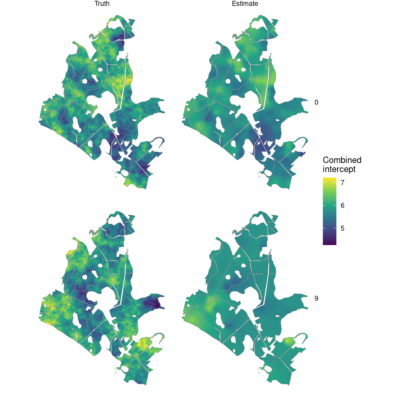
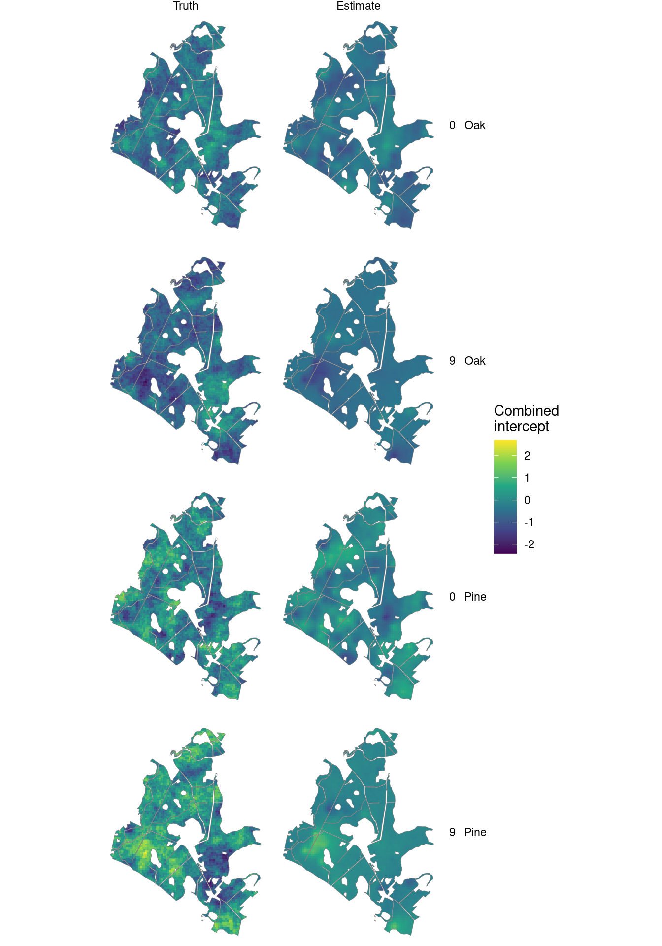
The maps compare combined intercepts at the first and last years. Each magnitude intercept is log density at average canopy height; the species intercepts are on the probit scale. The maps use the same latent draws as the density predictions.
intercept_summary <- summary(samples(predictions, type = "combined")) |>
  mutate(plot_id = as.integer(unit),
         component = if_else(component == "magnitude", "Magnitude", str_to_title(stick)))

true_intercepts <- prediction |>
  select(plot_id, location_id, year, magnitude_intercept, pine_intercept, oak_intercept) |>
  pivot_longer(ends_with("intercept"), names_to = "component", values_to = "truth") |>
  mutate(component = recode(component, magnitude_intercept = "Magnitude",
                             pine_intercept = "Pine", oak_intercept = "Oak"))

map_values <- intercept_summary |>
  select(plot_id, component, Estimate = mean) |>
  left_join(true_intercepts, by = c("plot_id", "component")) |>
  rename(Truth = truth) |>
  pivot_longer(c(Truth, Estimate), names_to = "source", values_to = "intercept") |>
  mutate(source = factor(source, levels = c("Truth", "Estimate")))

intercept_maps <- prediction_cells |>
  left_join(map_values, by = "location_id", relationship = "many-to-many")
Summarize each year’s forest distribution
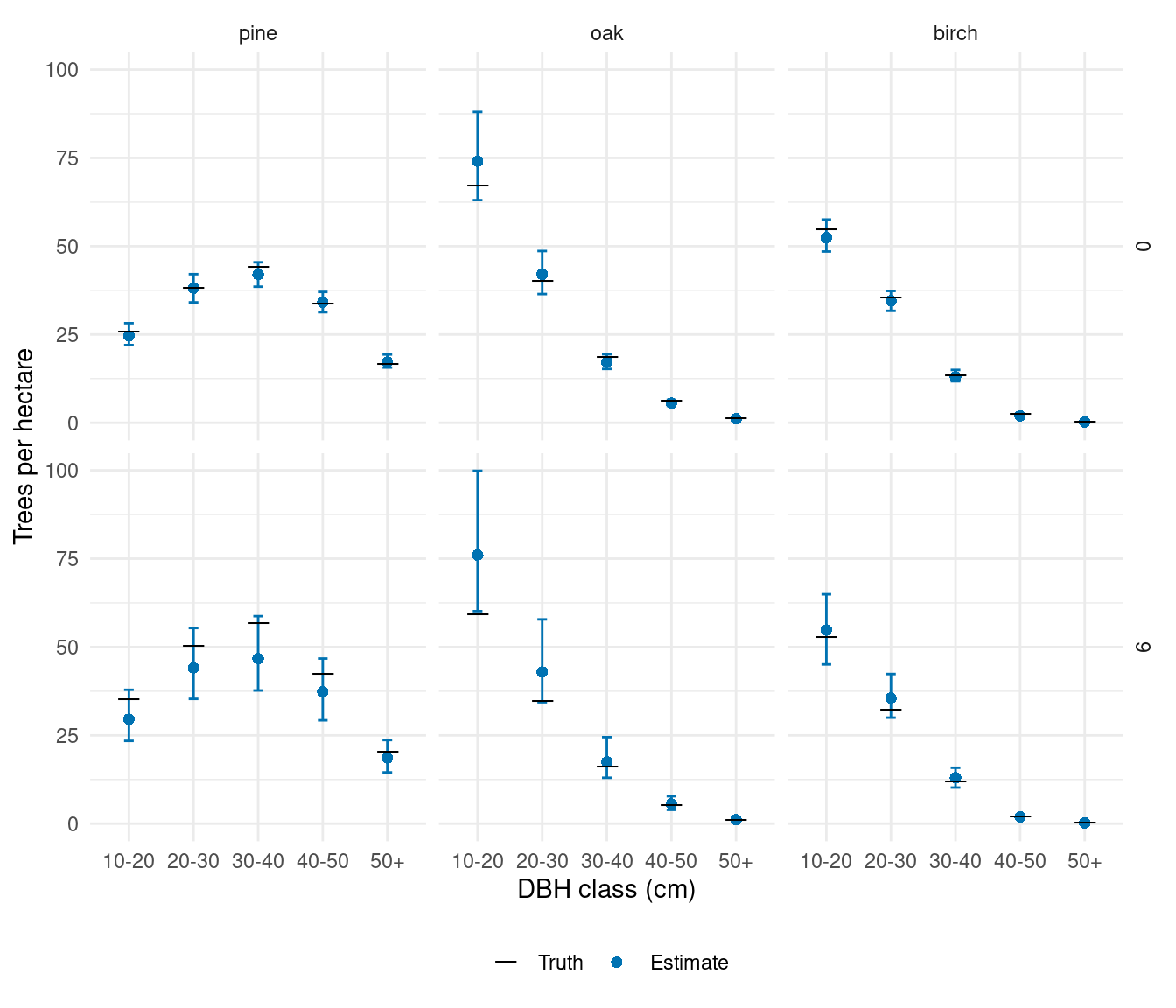
We pass year as the grouping variable to standSummary(). Each year gets its own area-weighted density, using the same forest cells. Omitting this group would average across both years, which is a different target.
forest_predictions <- standSummary(
  predictions, data = prediction, unit = plot_id, group = year,
  represented_area = area, summary = "samples"
)

forest_truth <- prediction |>
  select(year, area, contains(":")) |>
  pivot_longer(contains(":"), names_to = "category", values_to = "count") |>
  group_by(year, category) |>
  summarise(truth = sum(count) / sum(area), .groups = "drop")

forest_comparison <- summary(forest_predictions) |>
  as_tibble() |>
  mutate(year = as.integer(unit)) |>
  left_join(forest_truth, by = c("year", "category")) |>
  separate_wider_delim(category, delim = ":", names = c("species", "dbh_class")) |>
  mutate(species = factor(species, levels = species_order),
         dbh_class = ordered(dbh_class, levels = dbh_classes))
ggplot(forest_comparison, aes(dbh_class, mean)) +
  geom_errorbar(aes(ymin = q2_5, ymax = q97_5), width = 0.15, color = "#0072B2") +
  geom_point(aes(shape = "Estimate"), color = "#0072B2", size = 2) +
  geom_point(aes(y = truth, shape = "Truth"), size = 5) +
  scale_shape_manual(values = c("Truth" = 95, "Estimate" = 16),
                     breaks = c("Truth", "Estimate"), name = NULL) +
  facet_grid(year ~ species) +
  scale_y_continuous(limits = c(0, NA)) +
  labs(x = "DBH class (cm)", y = "Trees per hectare") +
  theme_minimal() +
  theme(legend.position = "bottom")
The year-9 intervals are generally wider: only 25 plots were measured in that year, and measurements from other years supply partial information through temporal dependence.
These distributions combine canopy height with the estimated space-time variation in abundance and species allocation. The model describes changing distributions; it does not track individual trees or impose a growth model. With time-varying canopy heights or other covariates, supply their values at each observed and prediction date. Stand summaries can use the same draws, with a grouping column that identifies each stand and year and the cell’s intersection area within that stand.
Spitta, Arthur, Andrew O. Finley, Christoph Gollob, Ralf Kraßnitzer, Tim Ritter, Andreas Tockner, and Arne Nothdurft. 2026.
“Evaluating LiDAR Data Sources, Predictor Resolution, and Spatial Random Effects in Bayesian Change-of-Support Models for Forest Inventory.” arXiv Preprint arXiv:2610.06476.
https://doi.org/10.48550/arXiv.2610.06476.