Function for Fitting Univariate Bayesian Spatial Regression Models

The function spNNGP fits Gaussian and non-Gaussian univariate Bayesian spatial regression models using Nearest Neighbor Gaussian Processes (NNGP).

Usage

spNNGP(formula, data = parent.frame(), coords, method = "response",
      family="gaussian", weights, n.neighbors = 15, 
      starting, tuning, priors, cov.model = "exponential",
      n.samples, n.omp.threads = 1, search.type = "cb", ord,
      return.neighbor.info = FALSE, neighbor.info,
      fit.rep = FALSE, sub.sample, verbose = TRUE, n.report = 100, ...)

Arguments

formula: a symbolic description of the regression model to be fit. See example below.
data: an optional data frame containing the variables in the model. If not found in data, the variables are taken from environment(formula), typically the environment from which spNNGP is called.
coords: an \(n \times 2\) matrix of the observation coordinates in \(R^2\) (e.g., easting and northing), or if data is a data frame then coords can be a vector of length two comprising coordinate column names or indices. There can be no duplicate locations.
method: a quoted keyword that specifies the NNGP sampling algorithm. Supported method keywords are: "response" and "latent". When \(n\) is large, the "response" algorithm should be faster and provide finer control over Metropolis acceptance rate for covariance parameters. In general, unless estimates of spatial random effects are needed, the "response" algorithm should be used.
family: a quoted keyword that specifies the data likelihood. Choices are "gaussian" for continuous outcome and "binomial" for discrete outcome which assumes a logistic link modeled using Polya-Gamma latent variables.
weights: specifies the number of trials for each observation when family="binomial". The default is 1 trial for each observation. Valid arguments are a scalar value that specifies the number of trials used if all observations have the same number of trials, and a vector of length \(n\) that specifies the number of trials for each observation used there are differences in the number of trials.
n.neighbors: number of neighbors used in the NNGP.
starting: a list with each tag corresponding to a parameter name. Valid tags are beta, sigma.sq, tau.sq, phi, and nu. nu is only specified if cov.model="matern". The value portion of each tag is the parameter's startingvalue.
tuning: a list with each tag corresponding to a parameter name. Valid tags are sigma.sq, tau.sq, phi, and nu. If method="latent" then only phi and nu need to be specified. The value portion of each tag defines the variance of the Metropolis sampler Normal proposal distribution.
priors: a list with each tag corresponding to a parameter name. Valid tags are sigma.sq.ig, tau.sq.ig, phi.unif, and nu.unif. Variance parameters, simga.sq and tau.sq, are assumed to follow an inverse-Gamma distribution, whereas the spatial decay phi and smoothness nu parameters are assumed to follow Uniform distributions. The hyperparameters of the inverse-Gamma are passed as a vector of length two, with the first and second elements corresponding to the shape and scale, respectively. The hyperparameters of the Uniform are also passed as a vector of length two with the first and second elements corresponding to the lower and upper support, respectively.
cov.model: a quoted keyword that specifies the covariance function used to model the spatial dependence structure among the observations. Supported covariance model key words are: "exponential", "matern", "spherical", and "gaussian". See below for details.
n.samples: the number of posterior samples to collect.
n.omp.threads: a positive integer indicating the number of threads to use for SMP parallel processing. The package must be compiled for OpenMP support. For most Intel-based machines, we recommend setting n.omp.threads up to the number of hyperthreaded cores. Note, n.omp.threads > 1 might not work on some systems.
fit.rep: if TRUE, regression fitted and replicate data will be returned. The argument sub.sample controls which MCMC samples are used to generate the fitted and replicated data.
sub.sample: an optional list that specifies the samples used for fit.rep. Valid tags are start, end, and thin. Given the value associated with the tags, the sample subset is selected using seq(as.integer(start), as.integer(end), by=as.integer(thin)). The default values are start=floor(0.5*n.samples), end=n.samples and thin=1.
verbose: if TRUE, model specification and progress of the sampler is printed to the screen. Otherwise, nothing is printed to the screen.
search.type: a quoted keyword that specifies type of nearest neighbor search algorithm. Supported method key words are: "cb" and "brute". The "cb" should generally be much faster. If locations do not have identical coordinate values on the axis used for the nearest neighbor ordering (see ord argument) then "cb" and "brute" should produce identical neighbor sets. However, if there are identical coordinate values on the axis used for nearest neighbor ordering, then "cb" and "brute" might produce different, but equally valid, neighbor sets, e.g., if data are on a grid.
ord: an index vector of length \(n\) used for the nearest neighbor search. Internally, this vector is used to order coords, i.e., coords[ord,], and associated data. Nearest neighbor candidates for the i-th row in the ordered coords are rows 1:(i-1), with the n.neighbors nearest neighbors being those with the minimum euclidean distance to the location defined by ordered coords[i,]. The default used when ord is not specified is x-axis ordering, i.e., order(coords[,1]). This argument should typically be left blank. This argument will be ignored if the neighbor.info argument is used.
return.neighbor.info: if TRUE, a list called neighbor.info containing several data structures used for fitting the NNGP model is returned. If there is no change in input data or n.neighbors, this list can be passed to subsequent spNNGP calls via the neighbor.info argument to avoid the neighbor search, which can be time consuming if \(n\) is large. In addition to the several cryptic data structures in neighbor.info there is a list called n.indx that is of length \(n\). The i-th element in n.indx corresponds to the i-th row in coords[ord,] and holds the vector of that location's nearest neighbor indices. This list can be useful for plotting the neighbor graph if desired.
neighbor.info: see the return.neighbor.info argument description above.
n.report: the interval to report Metropolis sampler acceptance and MCMC progress.
...: currently no additional arguments.

Value

An object of class NNGP with additional class designations for method and family. The return object is a list comprising:

p.beta.samples: a coda object of posterior samples for the regression coefficients.
p.theta.samples: a coda object of posterior samples for covariance parameters.
p.w.samples: is a matrix of posterior samples for the spatial random effects, where rows correspond to locations in coords and columns hold the n.samples posterior samples. This is only returned if method="latent".
y.hat.samples: if fit.rep=TRUE, regression fitted values from posterior samples specified using sub.sample. See additional details below.
y.hat.quants: if fit.rep=TRUE, 0.5, 0.025, and 0.975 quantiles of the y.hat.samples.
y.rep.samples: if fit.rep=TRUE, replicated outcome from posterior samples specified using sub.sample. See additional details below.
y.rep.quants: if fit.rep=TRUE, 0.5, 0.025, and 0.975 quantiles of the y.rep.samples.
s.indx: if fit.rep=TRUE, the subset index specified with sub.sample.
neighbor.info: returned if return.neighbor.info=TRUE see the return.neighbor.info argument description above.
run.time: execution time for parameter estimation reported using proc.time(). This time does not include nearest neighbor search time for building the neighbor set.

The return object will include additional objects used for subsequent prediction and/or model fit evaluation.

Details

Model parameters can be fixed at their starting values by setting their tuning values to zero.

The no nugget model is specified by setting tau.sq to zero in the starting and tuning lists.

References

Finley, A.O., A. Datta, S. Banerjee (2022) spNNGP R Package for Nearest Neighbor Gaussian Process Models. Journal of Statistical Software, doi:10.18637/jss.v103.i05 .

Datta, A., S. Banerjee, A.O. Finley, and A.E. Gelfand. (2016) Hierarchical Nearest-Neighbor Gaussian process models for large geostatistical datasets. Journal of the American Statistical Association, doi:10.1080/01621459.2015.1044091 .

Finley, A.O., A. Datta, B.D. Cook, D.C. Morton, H.E. Andersen, and S. Banerjee. (2019) Efficient algorithms for Bayesian Nearest Neighbor Gaussian Processes. Journal of Computational and Graphical Statistics, doi:10.1080/10618600.2018.1537924 .

Author

Andrew O. Finley finleya@msu.edu,
Abhirup Datta abhidatta@jhu.edu,
Sudipto Banerjee sudipto@ucla.edu

Examples


rmvn <- function(n, mu=0, V = matrix(1)){
  p <- length(mu)
  if(any(is.na(match(dim(V),p))))
    stop("Dimension problem!")
  D <- chol(V)
  t(matrix(rnorm(n*p), ncol=p)%*%D + rep(mu,rep(n,p)))
}

##Make some data
set.seed(1)
n <- 100
coords <- cbind(runif(n,0,1), runif(n,0,1))

x <- cbind(1, rnorm(n))

B <- as.matrix(c(1,5))

sigma.sq <- 5
tau.sq <- 1
phi <- 3/0.5

D <- as.matrix(dist(coords))
R <- exp(-phi*D)
w <- rmvn(1, rep(0,n), sigma.sq*R)
y <- rnorm(n, x%*%B + w, sqrt(tau.sq))

##Fit a Response and Latent NNGP model
n.samples <- 500

starting <- list("phi"=phi, "sigma.sq"=5, "tau.sq"=1)

tuning <- list("phi"=0.5, "sigma.sq"=0.5, "tau.sq"=0.5)

priors <- list("phi.Unif"=c(3/1, 3/0.01), "sigma.sq.IG"=c(2, 5), "tau.sq.IG"=c(2, 1))

cov.model <- "exponential"

m.s <- spNNGP(y~x-1, coords=coords, starting=starting, method="latent", n.neighbors=10,
              tuning=tuning, priors=priors, cov.model=cov.model,
              n.samples=n.samples, n.omp.threads=1)
#> ----------------------------------------
#> 	Building the neighbor list
#> ----------------------------------------
#> ----------------------------------------
#> Building the neighbors of neighbors list
#> ----------------------------------------
#> ----------------------------------------
#> 	Model description
#> ----------------------------------------
#> NNGP Latent model fit with 100 observations.
#> 
#> Number of covariates 2 (including intercept if specified).
#> 
#> Using the exponential spatial correlation model.
#> 
#> Using 10 nearest neighbors.
#> 
#> Number of MCMC samples 500.
#> 
#> Priors and hyperpriors:
#> 	beta flat.
#> 	sigma.sq IG hyperpriors shape=2.00000 and scale=5.00000
#> 	tau.sq IG hyperpriors shape=2.00000 and scale=1.00000
#> 	phi Unif hyperpriors a=3.00000 and b=300.00000
#> 
#> Source compiled with OpenMP support and model fit using 1 thread(s).
#> ----------------------------------------
#> 		Sampling
#> ----------------------------------------
#> Sampled: 100 of 500, 20.00%
#> Report interval Metrop. Acceptance rate: 52.00%
#> Overall Metrop. Acceptance rate: 52.00%
#> -------------------------------------------------
#> Sampled: 200 of 500, 40.00%
#> Report interval Metrop. Acceptance rate: 53.00%
#> Overall Metrop. Acceptance rate: 52.50%
#> -------------------------------------------------
#> Sampled: 300 of 500, 60.00%
#> Report interval Metrop. Acceptance rate: 52.00%
#> Overall Metrop. Acceptance rate: 52.33%
#> -------------------------------------------------
#> Sampled: 400 of 500, 80.00%
#> Report interval Metrop. Acceptance rate: 44.00%
#> Overall Metrop. Acceptance rate: 50.25%
#> -------------------------------------------------
#> Sampled: 500 of 500, 100.00%
#> Report interval Metrop. Acceptance rate: 56.00%
#> Overall Metrop. Acceptance rate: 51.40%
#> -------------------------------------------------

summary(m.s)
#> 
#> Call:
#> spNNGP(formula = y ~ x - 1, coords = coords, method = "latent", 
#>     n.neighbors = 10, starting = starting, tuning = tuning, priors = priors, 
#>     cov.model = cov.model, n.samples = n.samples, n.omp.threads = 1)
#> 
#> Model class is NNGP, method latent, family gaussian.
#> 
#> Model object contains 500 MCMC samples.
#> 
#> Chain sub.sample:
#> start = 250
#> end = 500
#> thin = 1
#> samples size = 251
#>          2.5%   25%     50%     75%     97.5%  
#> x1       1.4532 1.9494  2.1688  2.4433  2.7806 
#> x2       4.4950 4.6990  4.8426  4.9718  5.2373 
#> sigma.sq 2.3670 3.5773  4.1840  4.8601  6.5904 
#> tau.sq   0.2882 0.5759  0.7437  1.1290  2.0091 
#> phi      7.3423 10.2011 12.2097 15.6045 25.8783
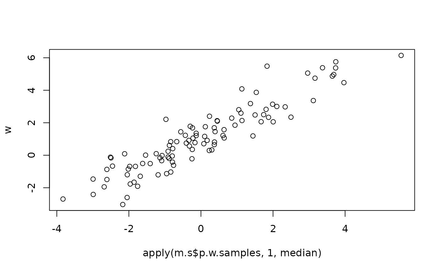
plot(apply(m.s$p.w.samples, 1, median), w)


m.r <- spNNGP(y~x-1, coords=coords, starting=starting, method="response", n.neighbors=10,
              tuning=tuning, priors=priors, cov.model=cov.model,
              n.samples=n.samples, n.omp.threads=1)
#> ----------------------------------------
#> 	Building the neighbor list
#> ----------------------------------------
#> ----------------------------------------
#> 	Model description
#> ----------------------------------------
#> NNGP Response model fit with 100 observations.
#> 
#> Number of covariates 2 (including intercept if specified).
#> 
#> Using the exponential spatial correlation model.
#> 
#> Using 10 nearest neighbors.
#> 
#> Number of MCMC samples 500.
#> 
#> Priors and hyperpriors:
#> 	beta flat.
#> 	sigma.sq IG hyperpriors shape=2.00000 and scale=5.00000
#> 	tau.sq IG hyperpriors shape=2.00000 and scale=1.00000
#> 	phi Unif hyperpriors a=3.00000 and b=300.00000
#> 
#> Source compiled with OpenMP support and model fit using 1 thread(s).
#> ----------------------------------------
#> 		Sampling
#> ----------------------------------------
#> Sampled: 100 of 500, 20.00%
#> Report interval Metrop. Acceptance rate: 33.00%
#> Overall Metrop. Acceptance rate: 33.00%
#> -------------------------------------------------
#> Sampled: 200 of 500, 40.00%
#> Report interval Metrop. Acceptance rate: 28.00%
#> Overall Metrop. Acceptance rate: 30.50%
#> -------------------------------------------------
#> Sampled: 300 of 500, 60.00%
#> Report interval Metrop. Acceptance rate: 29.00%
#> Overall Metrop. Acceptance rate: 30.00%
#> -------------------------------------------------
#> Sampled: 400 of 500, 80.00%
#> Report interval Metrop. Acceptance rate: 19.00%
#> Overall Metrop. Acceptance rate: 27.25%
#> -------------------------------------------------
#> Sampled: 500 of 500, 100.00%
#> Report interval Metrop. Acceptance rate: 23.00%
#> Overall Metrop. Acceptance rate: 26.40%
#> -------------------------------------------------

summary(m.r)
#> 
#> Call:
#> spNNGP(formula = y ~ x - 1, coords = coords, method = "response", 
#>     n.neighbors = 10, starting = starting, tuning = tuning, priors = priors, 
#>     cov.model = cov.model, n.samples = n.samples, n.omp.threads = 1)
#> 
#> Model class is NNGP, method response, family gaussian.
#> 
#> Model object contains 500 MCMC samples.
#> 
#> Chain sub.sample:
#> start = 250
#> end = 500
#> thin = 1
#> samples size = 251
#>          2.5%   25%    50%     75%     97.5%  
#> x1       1.1877 1.8342 2.1101  2.3642  2.9873 
#> x2       4.4913 4.7032 4.8236  4.9365  5.2016 
#> sigma.sq 1.7811 2.9784 3.3282  4.3400  7.5759 
#> tau.sq   0.2571 0.7788 1.1362  1.6107  2.1387 
#> phi      5.9495 8.0168 12.7328 15.3784 20.1438

##Fit with some user defined neighbor ordering

##ord <- order(coords[,2]) ##y-axis 
ord <- order(coords[,1]+coords[,2]) ##x+y-axis
##ord <- sample(1:n, n) ##random

m.r.xy <- spNNGP(y~x-1, coords=coords, starting=starting, method="response", n.neighbors=10,
              tuning=tuning, priors=priors, cov.model=cov.model,
              ord=ord, return.neighbor.info=TRUE,
              n.samples=n.samples, n.omp.threads=1)
#> ----------------------------------------
#> 	Building the neighbor list
#> ----------------------------------------
#> ----------------------------------------
#> 	Model description
#> ----------------------------------------
#> NNGP Response model fit with 100 observations.
#> 
#> Number of covariates 2 (including intercept if specified).
#> 
#> Using the exponential spatial correlation model.
#> 
#> Using 10 nearest neighbors.
#> 
#> Number of MCMC samples 500.
#> 
#> Priors and hyperpriors:
#> 	beta flat.
#> 	sigma.sq IG hyperpriors shape=2.00000 and scale=5.00000
#> 	tau.sq IG hyperpriors shape=2.00000 and scale=1.00000
#> 	phi Unif hyperpriors a=3.00000 and b=300.00000
#> 
#> Source compiled with OpenMP support and model fit using 1 thread(s).
#> ----------------------------------------
#> 		Sampling
#> ----------------------------------------
#> Sampled: 100 of 500, 20.00%
#> Report interval Metrop. Acceptance rate: 18.00%
#> Overall Metrop. Acceptance rate: 18.00%
#> -------------------------------------------------
#> Sampled: 200 of 500, 40.00%
#> Report interval Metrop. Acceptance rate: 19.00%
#> Overall Metrop. Acceptance rate: 18.50%
#> -------------------------------------------------
#> Sampled: 300 of 500, 60.00%
#> Report interval Metrop. Acceptance rate: 18.00%
#> Overall Metrop. Acceptance rate: 18.33%
#> -------------------------------------------------
#> Sampled: 400 of 500, 80.00%
#> Report interval Metrop. Acceptance rate: 32.00%
#> Overall Metrop. Acceptance rate: 21.75%
#> -------------------------------------------------
#> Sampled: 500 of 500, 100.00%
#> Report interval Metrop. Acceptance rate: 27.00%
#> Overall Metrop. Acceptance rate: 22.80%
#> -------------------------------------------------

summary(m.r.xy)
#> 
#> Call:
#> spNNGP(formula = y ~ x - 1, coords = coords, method = "response", 
#>     n.neighbors = 10, starting = starting, tuning = tuning, priors = priors, 
#>     cov.model = cov.model, n.samples = n.samples, n.omp.threads = 1, 
#>     ord = ord, return.neighbor.info = TRUE)
#> 
#> Model class is NNGP, method response, family gaussian.
#> 
#> Model object contains 500 MCMC samples.
#> 
#> Chain sub.sample:
#> start = 250
#> end = 500
#> thin = 1
#> samples size = 251
#>          2.5%   25%    50%     75%     97.5%  
#> x1       0.7771 1.6841 2.0819  2.4073  2.8944 
#> x2       4.4813 4.6922 4.8117  4.9609  5.1920 
#> sigma.sq 1.9662 3.5184 4.0121  4.9067  6.8949 
#> tau.sq   0.2933 0.6134 0.9782  1.4793  3.2605 
#> phi      3.6888 6.3814 10.2711 13.9859 18.4597

if (FALSE) { # \dontrun{
##Visualize the neighbor sets and ordering constraint
n.indx <- m.r.xy$neighbor.info$n.indx
ord <- m.r.xy$neighbor.info$ord

##This is how the data are ordered internally for model fitting
coords.ord <- coords[ord,]

for(i in 1:n){

    plot(coords.ord, cex=1, xlab="Easting", ylab="Northing")
    points(coords.ord[i,,drop=FALSE], col="blue", pch=19, cex=1)
    points(coords.ord[n.indx[[i]],,drop=FALSE], col="red", pch=19, cex=1)

    readline(prompt = "Pause. Press <Enter> to continue...")
}
} # }