
Areal CAR models with stLMM
County graphs, island handling, recovery, and holdout prediction
Source:vignettes/a01-areal-car.qmd
1 Overview
This vignette introduces areal spatial models using car() to fit conditional autoregressive (CAR) terms. To motivate this example, we use the bundled stunitco county polygon layer, extract Washington counties, build a county adjacency graph, simulate a Gaussian response from a proper CAR model, fit the model with a few county responses held out, recover the county random effects, and predict the held-out responses.
The key difference from point-referenced Gaussian process models is that the latent process is indexed by areal units (counties in this case) rather than coordinates. The graph defines which areas are neighbors, and the CAR precision matrix defines the dependence among area random effects.
2 Model
For area \(i\), the model is
\[ y_i = \beta_0 + x_i\beta_1 + w_i + \epsilon_i,\qquad \epsilon_i \sim N(0,\tau^2). \]
The default areal process is specified through the proper CAR precision matrix
\[ \mathbf{Q} = \sigma^{-2}(\mathbf{D} - \rho\mathbf{G}), \]
where \(\mathbf{G}\) is the binary adjacency matrix, \(\mathbf{D}\) is diagonal with entries equal to the number of neighbors for each area, \(\sigma^2\) controls the process variance, and \(\rho\) controls spatial association. The graph itself stores binary adjacency, but this degree-scaled precision is equivalent to a CAR conditional mean that averages neighboring effects. See Banerjee et al. (2014) for background on CAR models and hierarchical spatial modeling for areal data.
The same car_graph() object can also be used with car_model = "leroux", which gives the Leroux CAR precision \(\sigma^{-2}\{(1-\rho)\mathbf{I}+\rho(\mathbf{D}-\mathbf{G})\}\) (Leroux et al. 1999). This alternative is useful when the model should be able to move between nearly iid area effects and strong spatial smoothing using the same rho parameter. In this introductory example we use the default proper CAR model.
3 County graph
The stunitco object contains county polygons for the conterminous United States. Washington has one county that is not connected by polygon boundaries to the rest of the state graph, so the default graph-building rule reports the issue in the error below. For this vignette, we make the island rule explicit and add nearest-neighbor bridge edges.
Code
data(stunitco, package = "stLMM")

wa_counties <- stunitco[stunitco$STATECD == 53, ]
Code
car_graph(wa_counties, id = "COUNTYFIPS")Error in `car_graph()`:
! error: CAR graph contains isolated area(s): 53055Now, let’s correct the island issue using the nearest-neighbor bridge rule in the code below. Here, setting island_k = 4 adds four nearest-neighbor bridge edges from the disconnected component.
Code
g <- car_graph(wa_counties, id = "COUNTYFIPS", island = "nearest", island_k = 4)

g$island_added_edges
from to distance
1 53055 53029 56295.36
2 53055 53035 100454.10
3 53055 53073 100817.65
4 53055 53057 102288.17The graph object stores county IDs, binary adjacency, node degrees, and any bridge edges added by the island rule. The graph is not stored as a row-standardized matrix; the neighbor averaging enters through the degree-scaled CAR precision.
Show edge-map code
coord_dat <- data.frame(
  area = as.character(wa_counties$COUNTYFIPS),
  sf::st_coordinates(
    sf::st_point_on_surface(sf::st_geometry(wa_counties))
  )
)

edge_index <- which(as.matrix(g$adjacency) != 0, arr.ind = TRUE)
edge_index <- edge_index[edge_index[, "row"] < edge_index[, "col"], , drop = FALSE]
edge_dat <- data.frame(
  from = g$ids[edge_index[, "row"]],
  to = g$ids[edge_index[, "col"]]
)
edge_dat$key <- paste(
  pmin(edge_dat$from, edge_dat$to),
  pmax(edge_dat$from, edge_dat$to),
  sep = "--"
)
edge_dat$x <- coord_dat$X[match(edge_dat$from, coord_dat$area)]
edge_dat$y <- coord_dat$Y[match(edge_dat$from, coord_dat$area)]
edge_dat$xend <- coord_dat$X[match(edge_dat$to, coord_dat$area)]
edge_dat$yend <- coord_dat$Y[match(edge_dat$to, coord_dat$area)]

island_key <- paste(
  pmin(g$island_added_edges$from, g$island_added_edges$to),
  pmax(g$island_added_edges$from, g$island_added_edges$to),
  sep = "--"
)
edge_dat$island <- edge_dat$key %in% island_key

ggplot(wa_counties) +
  geom_sf(
    fill = "grey95",
    color = "white",
    linewidth = 0.15
  ) +
  geom_segment(
    data = edge_dat,
    aes(x = x, y = y, xend = xend, yend = yend, color = island, linewidth = island)
  ) +
  geom_point(
    data = coord_dat,
    aes(X, Y),
    color = stlmm_color("primary"),
    size = 1.4
  ) +
  scale_color_manual(
    values = c("FALSE" = "grey45", "TRUE" = stlmm_color("secondary")),
    guide = "none"
  ) +
  scale_linewidth_manual(
    values = c("FALSE" = 0.25, "TRUE" = 1),
    guide = "none"
  ) +
  labs(x = "longitude", y = "latitude")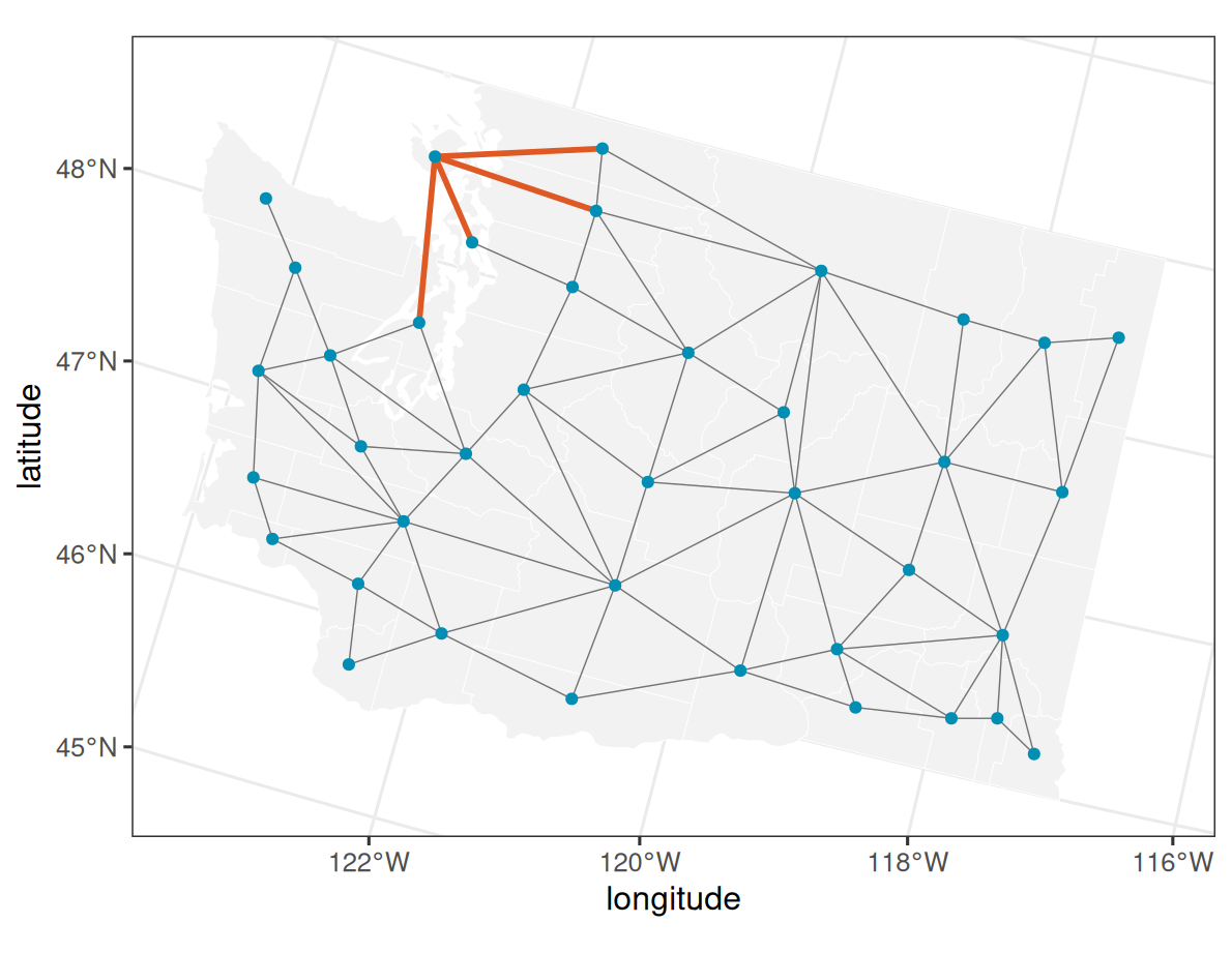
4 Data
We construct a simple county-level covariate from the east-west position of each polygon. This is only for simulation; it gives the fixed-effect part of the model a visible spatial trend. Following the model statement, the CAR dependence is parameterized through the precision matrix \(\mathbf{Q}\). However, in the simulation code below, rmvnorm() draws from a covariance matrix, so we compute \(\mathbf{\Sigma} = \mathbf{Q}^{-1}\) before drawing the county effects.
Code
centroid_x <- sf::st_coordinates(sf::st_centroid(sf::st_geometry(wa_counties)))[, "X"]
centroid_x_mean <- mean(centroid_x)
centroid_x_sd <- stats::sd(centroid_x)

dat <- data.frame(
  area = as.character(wa_counties$COUNTYFIPS),
  county = wa_counties$COUNTYNM,
  x = (centroid_x - centroid_x_mean) / centroid_x_sd
)

beta <- c(0.5, -1)
sigma_sq <- 1
rho <- 0.75
tau_sq <- 0.1

Q <- car_prec(g, sigma_sq = sigma_sq, rho = rho)
Sigma <- solve(Q)

w <- rmvnorm(mean = rep(0, nrow(Q)), Sigma = Sigma)
names(w) <- rownames(Q)

dat$w_true <- w[dat$area]

mu <- beta[1] + beta[2] * dat$x + dat$w_true
epsilon <- rnorm(nrow(dat), sd = sqrt(tau_sq))
dat$y_full <- mu + epsilon

holdout_id <- sample(seq_len(nrow(dat)), 6)
dat$sample <- "training"
dat$sample[holdout_id] <- "holdout"

dat$y <- dat$y_full
dat$y[holdout_id] <- NA
The CAR county-level smoothing and the east-west covariate trend are apparent in the mapped response values below.
Show plotting code
wa_plot <- wa_counties
wa_plot$area <- as.character(wa_plot$COUNTYFIPS)
wa_plot$y_full <- dat$y_full[match(wa_plot$area, dat$area)]
wa_plot$sample <- dat$sample[match(wa_plot$area, dat$area)]

ggplot(wa_plot) +
  geom_sf(
    aes(fill = y_full),
    color = "white",
    linewidth = 0.15
  ) +
  geom_sf(
    data = wa_plot[wa_plot$sample == "holdout", ],
    fill = NA,
    color = "black",
    linewidth = 0.8
  ) +
  scale_fill_gradientn(colors = stlmm_palette()) +
  labs(fill = "response")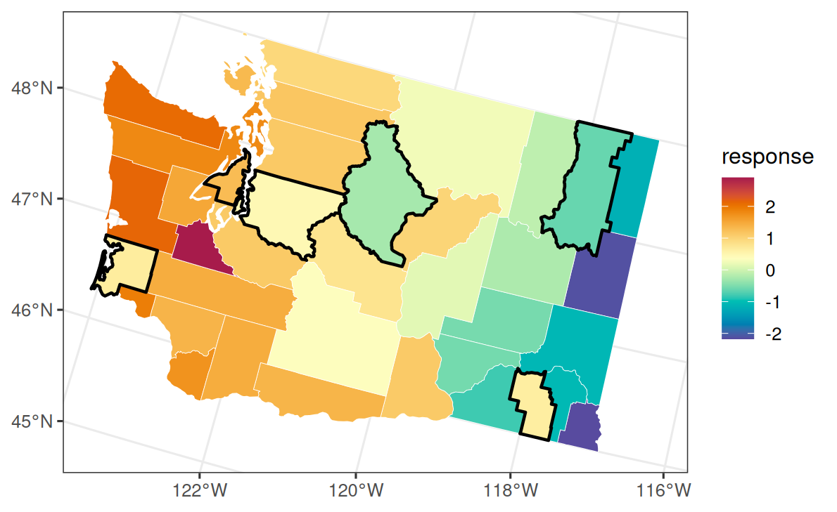
5 Fit
Rows with y = NA are included in the fitting data so that the fitted graph still contains the held-out counties. They do not contribute to the likelihood, but they remain available for recovery and prediction because their county IDs are part of the CAR support.
The residual and process variances use half-\(t\) priors on their corresponding standard deviations. The CAR association parameter rho uses a bounded uniform prior over positive spatial association values.
Code
stLMM summary
  formula: y ~ x + car(area, graph = g)
  observations: 39 (33 observed, 6 missing response)
  posterior draws: 500
  family: gaussian
  fixed effects: 2
  grouped random-effect coefficients: 0
  process terms: 1
  residual variance: global tau_sq

beta:
               mean     sd    q2.5   q50.0   q97.5
(Intercept)  0.6432 0.1309  0.3605  0.6499  0.9146
x           -1.1290 0.1308 -1.3928 -1.1269 -0.8788

tau_sq:
        mean    sd q2.5  q50.0  q97.5
value 0.0663 0.071    0 0.0363 0.2506

sigma_sq:
                 mean     sd   q2.5  q50.0  q97.5
car_1_sigma_sq 0.8707 0.3614 0.3245 0.8297 1.7979

theta:
            mean     sd   q2.5  q50.0  q97.5
car_1_rho 0.4686 0.2597 0.0659 0.4468 0.9155
6 Recover
Like other structured process terms, CAR effects are integrated out during fitting. Calling recover() draws the county-level CAR effects conditional on the posterior parameter samples.
stLMM recovery
  formula: y ~ x + car(area, graph = g)
  observations: 39 (33 observed, 6 missing response)
  recovered draws: 176
  recovered process terms: car_1
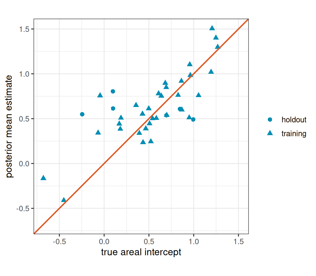
The recovered car_1 columns are ordered according to g$ids. As in the point-referenced spatial vignette, the data identify the combined areal intercept, \(\beta_0 + w_i\), more directly than the split between the global intercept and the average level of one realized areal process. For this diagnostic, we therefore compare \(\beta_0 + w_i\) rather than \(w_i\) alone.
Show plotting code
rec_draws <- as_samples(rec, include_w = TRUE, metadata = FALSE)
w_cols <- paste0("w_car_1_", seq_along(g$ids))
w_hat <- colMeans(rec_draws[, w_cols, drop = FALSE])
names(w_hat) <- g$ids
beta_0_hat <- mean(rec_draws[["(Intercept)"]])

recovery_dat <- data.frame(
  truth = beta[1] + dat$w_true,
  estimate = beta_0_hat + w_hat[dat$area],
  sample = dat$sample
)
recovery_lim <- range(recovery_dat$truth, recovery_dat$estimate)

ggplot(recovery_dat, aes(truth, estimate)) +
  geom_point(
    aes(shape = sample),
    color = stlmm_color("primary"),
    size = 2.2
  ) +
  geom_abline(
    intercept = 0,
    slope = 1,
    color = stlmm_color("secondary"),
    linewidth = 0.8
  ) +
  coord_equal(
    xlim = recovery_lim,
    ylim = recovery_lim
  ) +
  labs(
    x = "true areal intercept",
    y = "posterior mean estimate",
    shape = NULL
  )
7 Predict
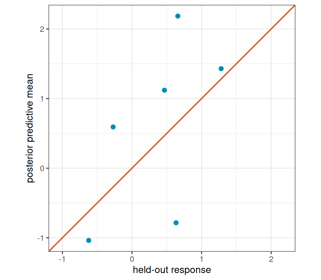
CAR prediction uses areas that already belong to the fitted graph. Here the held-out counties were included in the original data with y = NA, so they can be predicted after recovery.
Code
stLMM prediction summary
  draws: 176
  rows: 6
  newdata: TRUE
  process samples: car_1

mu:
      mean     sd    q2.5   q50.0   q97.5
22 -0.7699 0.5202 -1.6667 -0.7632  0.3207
6   0.6345 0.4595 -0.3448  0.6552  1.5291
28  2.2056 0.5891  1.0587  2.1762  3.2496
3   1.1151 0.4556  0.2410  1.0732  1.9980
39 -1.0433 0.5030 -1.9760 -1.0728 -0.0964
7   1.4486 0.5448  0.4082  1.4496  2.5277

y:
      mean     sd    q2.5   q50.0   q97.5
22 -0.7842 0.5817 -1.9058 -0.7870  0.4519
6   0.5924 0.5359 -0.4493  0.6094  1.6460
28  2.1853 0.6335  0.9590  2.1734  3.4017
3   1.1205 0.5183  0.0420  1.1239  2.0144
39 -1.0380 0.5259 -2.0603 -1.0538 -0.0563
7   1.4294 0.5992  0.2144  1.4256  2.7018
The predict() call returns posterior draws of \(\mu\) in mu_samples and, because y_samples = TRUE, posterior predictive response draws in y_samples. Passing the prediction object to summary() gives posterior summaries for these draws.
Show plotting code
pred_y <- as_samples(pred, sample = "y", metadata = FALSE)
pred_dat <- data.frame(
  y = dat$y_full[holdout_id],
  y_hat = colMeans(pred_y)
)
pred_lim <- range(pred_dat$y, pred_dat$y_hat)

ggplot(pred_dat, aes(y, y_hat)) +
  geom_point(
    color = stlmm_color("primary"),
    size = 2.2
  ) +
  geom_abline(
    intercept = 0,
    slope = 1,
    color = stlmm_color("secondary"),
    linewidth = 0.8
  ) +
  coord_equal(
    xlim = pred_lim,
    ylim = pred_lim
  ) +
  labs(
    x = "held-out response",
    y = "posterior predictive mean"
  )
8 What this example illustrates
The car() term is for areal data where the latent process is indexed by graph nodes. The graph, not Euclidean distance, defines neighboring areas. Prediction is therefore different from point-referenced NNGP prediction: a CAR model can predict existing areas in the fitted graph, including areas whose responses were held out with NA, but it does not create new areas outside the graph.
9 Choosing a CAR precision
The default car() term uses the package’s original degree-scaled proper CAR precision. The same graph can also be used with the Leroux CAR precision (Leroux et al. 1999):
The Leroux option is useful when rho should describe a transition from nearly iid area effects to strong spatial smoothing. Both choices use the same car_graph() object, the same process variance parameter sigma_sq, and the same rho prior, starting, and tuning structure. The exact intrinsic-CAR endpoint rho = 1 is not included; use an upper prior bound below one, such as uniform(0.01, 0.99).