
Areal DAGAR models with stLMM
Directed areal graphs, ordering, recovery, and holdout prediction
Source:vignettes/a02-areal-dagar.qmd
1 Overview
This vignette introduces directed acyclic graph autoregressive (DAGAR) areal models using dagar(). We use Washington counties from stunitco, build a county adjacency graph, convert that undirected graph into an ordered directed graph, simulate a Gaussian response from a DAGAR latent effect, fit the model with a few county responses held out, recover the county random effects, and predict the held-out responses.
DAGAR models were developed by Datta et al. (2019) as an alternative to common conditional autoregressive (CAR) models for areal spatial smoothing. The starting point is still an areal neighborhood graph, but dependence is represented through a directed acyclic graph (DAG) induced by an ordering of the areal units. This makes the ordering part of the spatial model specification, not just a computational detail.
2 Model
For area \(i\), the observation model is
\[ y_i = \beta_0 + x_i\beta_1 + w_i + \epsilon_i,\qquad \epsilon_i \sim N(0,\tau^2). \]
The DAGAR prior is built from an undirected areal graph and an ordering of its areas. Let \(N_\pi(i)\) be the set of directed parents of ordered area \(i\) and let \(m_i = |N_\pi(i)|\). Under the DAGAR model used by stLMM,
\[ w_i \mid \{w_j:j\in N_\pi(i)\} \sim N\left( \frac{\rho}{1 + (m_i - 1)\rho^2} \sum_{j\in N_\pi(i)}w_j,\, \sigma^2\frac{1-\rho^2}{1 + (m_i - 1)\rho^2} \right). \]
If an ordered area has no parents, the conditional mean is zero and the conditional variance is \(\sigma^2\). The parameter \(\sigma^2\) controls the marginal scale of the areal process, while \(\rho\) controls positive spatial association along the directed parent graph. The implemented model supports \(0 \le \rho < 1\); in this example we use a prior bounded away from the endpoints.
The equivalent precision matrix can be written as
\[ \mathbf{Q}_{\mathrm{dagar}} = \sigma^{-2}\mathbf{L}_{\pi}^{\top}\mathbf{F}_{\pi}\mathbf{L}_{\pi}, \]
where \(\mathbf{L}_{\pi}\) contains the directed parent coefficients and \(\mathbf{F}_{\pi}\) contains the conditional precisions. This is the sparse precision used internally by stLMM.
3 County graph and ordering
The stunitco object contains county polygons for the conterminous United States. Washington has one county that is not connected by polygon boundaries to the rest of the state graph, so we use the same nearest-neighbor bridge rule used in the areal CAR vignette.
Code
   from    to  distance
1 53055 53029  56295.36
2 53055 53035 100454.10
3 53055 53073 100817.65
4 53055 53057 102288.17
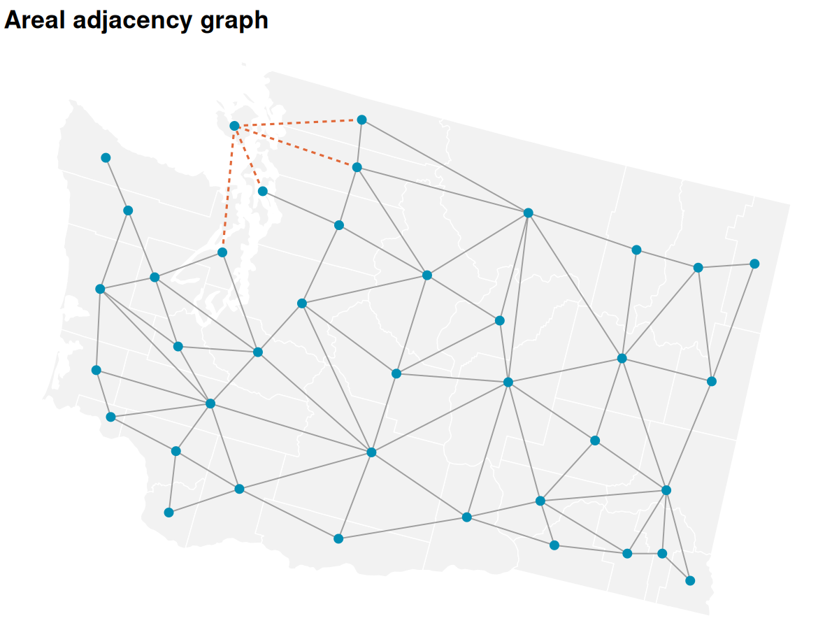
The undirected graph defines which counties can become DAGAR parent-child pairs. The ordering determines the direction of each eligible edge. For areal graphs built from sf polygons, ordering = "coord" orders the counties by their point-on-surface coordinates, ordering = "maxmin" uses a spatial max-min ordering, ordering = "hilbert" uses a Hilbert curve ordering, and ordering = "random" samples an ordering.
The plot below shows the undirected adjacency graph. Bridge edges added for the island county are shown as dashed lines.
Show graph plotting code
plot(
  g,
  show_nodes = TRUE,
  show_bridges = TRUE,
  edge_color = "grey45",
  bridge_color = stlmm_color("secondary"),
  node_color = stlmm_color("primary")
)
For simulation, we construct the ordered DAGAR precision using ordering = "coord". The helper dagar_prec() in utils.R follows the same DAGAR precision formula used by the package and stores the ordered graph as an attribute so we can visualize it.
Code
sigma_sq <- 1
rho <- 0.7

Q <- dagar_prec(g, sigma_sq = sigma_sq, rho = rho, ordering = "coord")
dg <- attr(Q, "dagar_graph")
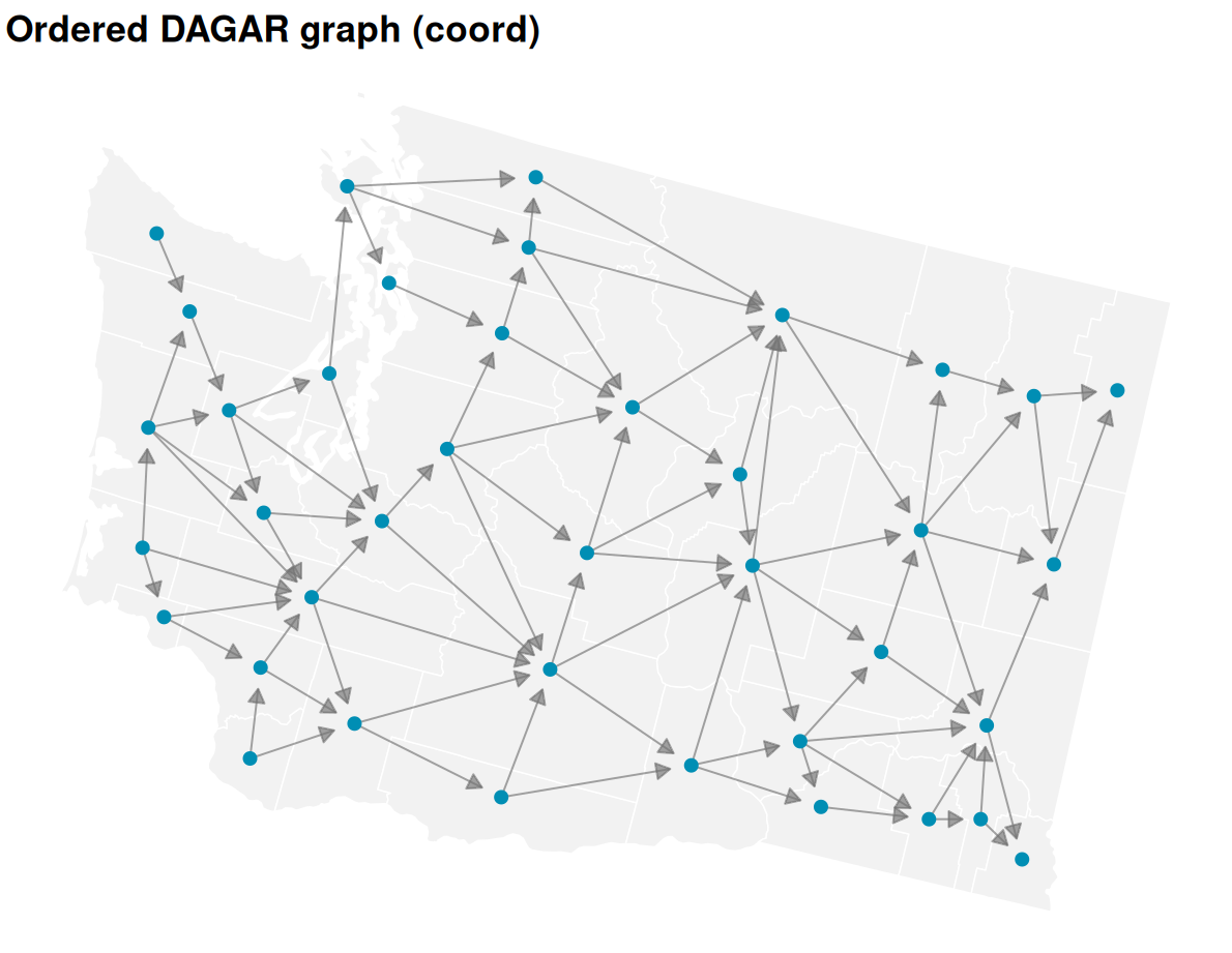
The directed graph plot shows the parent edges after ordering. Arrows point from parents to children, so each county can depend only on counties earlier in the ordering.
Show directed graph plotting code
plot(
  dg,
  show_nodes = TRUE,
  edge_color = "grey45",
  node_color = stlmm_color("primary")
)
4 Data
We construct a county-level covariate from the east-west position of each polygon. This is only for simulation; it gives the fixed-effect part of the model a visible spatial trend. The DAGAR dependence is parameterized through the precision matrix \(\mathbf{Q}\). However, in the simulation code below, rmvnorm() draws from a covariance matrix, so we compute \(\mathbf{\Sigma} = \mathbf{Q}^{-1}\) before drawing the county effects.
Code
centroid_x <- sf::st_coordinates(sf::st_centroid(sf::st_geometry(wa_counties)))[, "X"]
centroid_x_mean <- mean(centroid_x)
centroid_x_sd <- stats::sd(centroid_x)

dat <- data.frame(
  area = as.character(wa_counties$COUNTYFIPS),
  county = wa_counties$COUNTYNM,
  x = (centroid_x - centroid_x_mean) / centroid_x_sd
)

beta <- c(0.5, -1)
tau_sq <- 0.1

Sigma <- solve(Q)
w <- rmvnorm(mean = rep(0, nrow(Q)), Sigma = Sigma)
names(w) <- rownames(Q)

dat$w_true <- w[dat$area]

mu <- beta[1] + beta[2] * dat$x + dat$w_true
epsilon <- rnorm(nrow(dat), sd = sqrt(tau_sq))
dat$y_full <- mu + epsilon

holdout_id <- sample(seq_len(nrow(dat)), 6)
dat$sample <- "training"
dat$sample[holdout_id] <- "holdout"

dat$y <- dat$y_full
dat$y[holdout_id] <- NA
The mapped response values show the east-west covariate trend plus county-level DAGAR variation. The black outlines mark counties held out from the likelihood.
Show plotting code
wa_plot <- wa_counties
wa_plot$area <- as.character(wa_plot$COUNTYFIPS)
wa_plot$y_full <- dat$y_full[match(wa_plot$area, dat$area)]
wa_plot$sample <- dat$sample[match(wa_plot$area, dat$area)]

ggplot(wa_plot) +
  geom_sf(
    aes(fill = y_full),
    color = "white",
    linewidth = 0.15
  ) +
  geom_sf(
    data = wa_plot[wa_plot$sample == "holdout", ],
    fill = NA,
    color = "black",
    linewidth = 0.8
  ) +
  scale_fill_gradientn(colors = stlmm_palette()) +
  labs(fill = "response")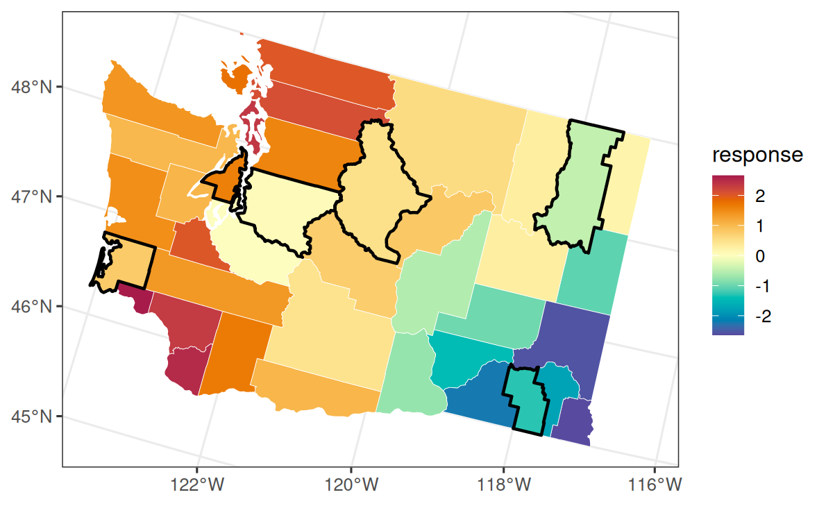
5 Fit
Rows with y = NA are included in the fitting data so that the fitted graph still contains the held-out counties. They do not contribute to the likelihood, but they remain available for recovery and prediction because their county IDs are part of the DAGAR support.
The residual and process variances use half-\(t\) priors on their corresponding standard deviations. The DAGAR association parameter rho uses a bounded uniform prior over positive spatial association values.
Code
stLMM summary
  formula: y ~ x + dagar(area, graph = g, ordering = "coord")
  observations: 39 (33 observed, 6 missing response)
  posterior draws: 500
  family: gaussian
  fixed effects: 2
  grouped random-effect coefficients: 0
  process terms: 1
  residual variance: global tau_sq

beta:
               mean     sd    q2.5   q50.0   q97.5
(Intercept)  1.2027 0.5821  0.1441  1.2061  2.4913
x           -1.0507 0.2866 -1.6403 -1.0479 -0.5215

tau_sq:
        mean     sd q2.5  q50.0  q97.5
value 0.0315 0.0471    0 0.0119 0.1669

sigma_sq:
                   mean     sd   q2.5 q50.0  q97.5
dagar_1_sigma_sq 1.1192 0.5926 0.4568  0.99 2.7247

theta:
              mean     sd   q2.5  q50.0  q97.5
dagar_1_rho 0.6505 0.1143 0.4598 0.6519 0.8698
6 Recover
Like other structured process terms, DAGAR effects are integrated out during fitting. Calling recover() draws the county-level DAGAR effects conditional on the posterior parameter samples.
stLMM recovery
  formula: y ~ x + dagar(area, graph = g, ordering = "coord")
  observations: 39 (33 observed, 6 missing response)
  recovered draws: 176
  recovered process terms: dagar_1
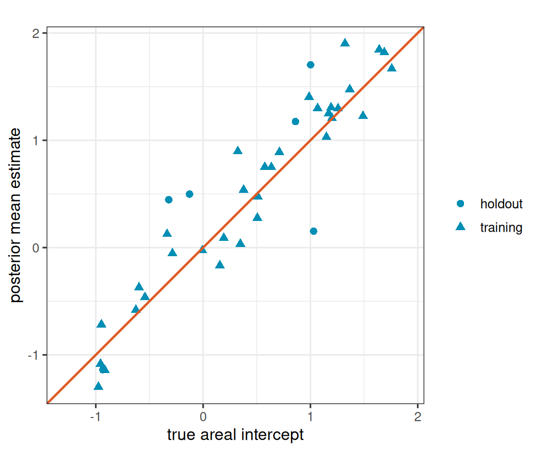
The recovered dagar_1 columns are returned in the original graph support order. As in the CAR and NNGP vignettes, the data identify the combined areal intercept, \(\beta_0 + w_i\), more directly than the split between the global intercept and the average level of one realized areal process. For this diagnostic, we therefore compare \(\beta_0 + w_i\) rather than \(w_i\) alone.
Show plotting code
rec_draws <- as_samples(rec, include_w = TRUE, metadata = FALSE)
w_cols <- paste0("w_dagar_1_", seq_along(g$ids))
w_hat <- colMeans(rec_draws[, w_cols, drop = FALSE])
names(w_hat) <- g$ids
beta_0_hat <- mean(rec_draws[["(Intercept)"]])

recovery_dat <- data.frame(
  truth = beta[1] + dat$w_true,
  estimate = beta_0_hat + w_hat[dat$area],
  sample = dat$sample
)
recovery_lim <- range(recovery_dat$truth, recovery_dat$estimate)

ggplot(recovery_dat, aes(truth, estimate)) +
  geom_point(
    aes(shape = sample),
    color = stlmm_color("primary"),
    size = 2.2
  ) +
  geom_abline(
    intercept = 0,
    slope = 1,
    color = stlmm_color("secondary"),
    linewidth = 0.8
  ) +
  coord_equal(
    xlim = recovery_lim,
    ylim = recovery_lim
  ) +
  labs(
    x = "true areal intercept",
    y = "posterior mean estimate",
    shape = NULL
  )
7 Predict
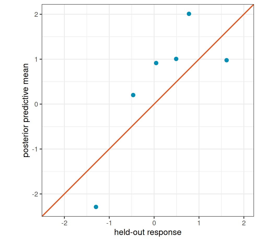
DAGAR prediction uses areas that already belong to the fitted graph. Here the held-out counties were included in the original data with y = NA, so they can be predicted after recovery.
Code
stLMM prediction summary
  draws: 176
  rows: 6
  newdata: TRUE
  process samples: dagar_1

mu:
      mean     sd    q2.5   q50.0   q97.5
22 -2.2807 0.5981 -3.4847 -2.3202 -0.9721
6   1.0202 0.4800  0.2455  0.9870  1.9756
28  1.9998 0.5711  0.6804  2.0022  3.0613
3   0.9003 0.5842 -0.1319  0.8870  2.0106
39  0.2068 0.5201 -0.6500  0.1932  1.1977
7   0.9779 0.6290 -0.2103  0.9865  2.1848

y:
      mean     sd    q2.5   q50.0   q97.5
22 -2.2894 0.6062 -3.4059 -2.3121 -1.1045
6   1.0060 0.5269  0.2022  0.9706  1.9693
28  2.0097 0.5898  0.6855  1.9655  3.1335
3   0.9140 0.6362 -0.1232  0.8901  2.0629
39  0.2014 0.5523 -0.7511  0.1612  1.2072
7   0.9770 0.6910 -0.2628  0.9885  2.3631
The predict() call returns posterior draws of the conditional mean \(\mu\) in mu_samples and, because y_samples = TRUE, posterior predictive response draws in y_samples.
Show plotting code
pred_y <- as_samples(pred, sample = "y", metadata = FALSE)
pred_dat <- data.frame(
  y = dat$y_full[holdout_id],
  y_hat = colMeans(pred_y)
)
pred_lim <- range(pred_dat$y, pred_dat$y_hat)

ggplot(pred_dat, aes(y, y_hat)) +
  geom_point(
    color = stlmm_color("primary"),
    size = 2.2
  ) +
  geom_abline(
    intercept = 0,
    slope = 1,
    color = stlmm_color("secondary"),
    linewidth = 0.8
  ) +
  coord_equal(
    xlim = pred_lim,
    ylim = pred_lim
  ) +
  labs(
    x = "held-out response",
    y = "posterior predictive mean"
  )
8 Ordering guidance
The ordering determines which undirected neighbor edges become directed parent edges. Coordinate-based, max-min, and Hilbert orderings are useful defaults when the graph comes from areal geometry. A user-supplied permutation is also allowed when the application has a meaningful ordering, such as a known direction of propagation or a fixed historical convention.
Different orderings define different DAGAR precision matrices, so they can produce different posterior summaries. This is part of the model definition. In practice, it is useful to compare a small number of scientifically reasonable orderings and check whether substantive conclusions are stable.
We refit the same model under these three orderings and compare posterior summaries for the fixed effects, residual variance, process variance, and DAGAR association parameter. In an applied analysis, this kind of comparison is a useful sensitivity check: the goal is not to choose an ordering because it gives the most convenient answer, but to learn whether the scientific conclusions depend strongly on this part of the model specification.
Code
fit_dagar_ordering <- function(ordering){
  stLMM(
    y ~ x + dagar(area, graph = g, ordering = ordering),
    data = dat,
    priors = list(
      resid = list(tau_sq = half_t(df = 3, scale = 0.5)),
      dagar_1 = list(
        sigma_sq = half_t(df = 3, scale = 1),
        rho = uniform(0.05, 0.95)
      )
    ),
    n_samples = 350,
    verbose = FALSE
  )
}

ordering_fits <- lapply(
  c("coord", "maxmin", "hilbert"),
  fit_dagar_ordering
)
names(ordering_fits) <- c("coord", "maxmin", "hilbert")

ordering_table <- do.call(
  rbind,
  lapply(names(ordering_fits), function(ordering){
    fit_i <- ordering_fits[[ordering]]
    samples <- as_samples(fit_i, burn = 150, metadata = FALSE)
    samples <- samples[, c("(Intercept)", "x", "tau_sq", "dagar_1_sigma_sq", "dagar_1_rho")]
    names(samples)[4:5] <- c("sigma_sq", "rho")
    summ <- t(apply(samples, 2, function(x){
      stats::quantile(x, probs = c(0.025, 0.5, 0.975))
    }))

    data.frame(
      ordering = ordering,
      parameter = rownames(summ),
      q2.5 = round(summ[, 1], 3),
      median = round(summ[, 2], 3),
      q97.5 = round(summ[, 3], 3),
      row.names = NULL
    )
  })
)

ordering_table
ordering parameter q2.5 median q97.5
1 coord (Intercept) 0.278 1.170 2.412
2 coord x -1.607 -1.027 -0.502
3 coord tau_sq 0.000 0.011 0.151
4 coord sigma_sq 0.602 0.973 2.174
5 coord rho 0.546 0.677 0.826
6 maxmin (Intercept) 0.078 0.546 1.052
7 maxmin x -1.752 -1.227 -0.709
8 maxmin tau_sq 0.027 0.203 0.473
9 maxmin sigma_sq 0.409 0.953 1.489
10 maxmin rho 0.325 0.757 0.884
11 hilbert (Intercept) 0.459 1.192 2.131
12 hilbert x -1.809 -1.264 -0.730
13 hilbert tau_sq 0.000 0.029 0.154
14 hilbert sigma_sq 0.563 1.014 2.861
15 hilbert rho 0.407 0.683 0.868The table is not meant to identify a best ordering. It is meant to show whether the main fixed-effect and variance conclusions are broadly stable across reasonable graph orderings.
9 Extensions
The space-time DAGAR term replaces the CAR spatial component in car_time() with a DAGAR spatial component. The time component and data layout follow the same rules as the space-time CAR vignettes. The example below shows the syntax for an areal response indexed by area and time.
Use time_model = "exp" when the fitted time support is numeric and temporal association should depend on actual time gaps.
Code
fit_dagar_time_exp <- stLMM(
  y ~ x + dagar_time(area, decimal_year, graph = g,
                    ordering = "coord", time_model = "exp"),
  data = dat,
  priors = list(
    resid = list(tau_sq = half_t(df = 3, scale = 0.5)),
    dagar_time_1 = list(
      sigma_sq = half_t(df = 3, scale = 1),
      rho = uniform(0.05, 0.95),
      lambda = log_normal(meanlog = 0, sdlog = 1)
    )
  )
)
Point observations can also be linked to an areal DAGAR or DAGAR-time support. In that case, each point-level row carries the associated area ID, and multiple point observations can share the same areal latent effect. If you want a random effect or prediction for an area, time, or area-time cell with no observed point rows, include a row with y = NA and the associated area, time, and covariate values.
10 What this example illustrates
The dagar() term is for areal data where the latent process is indexed by graph nodes and the graph is converted into an ordered directed parent graph. Prediction is for existing areas in the fitted graph, including areas whose responses were held out with NA. The main DAGAR-specific choices are the areal graph and the ordering used to orient that graph.