
Space-time CAR models with stLMM
Areal space-time effects, recovery, and holdout prediction
Source:vignettes/a03-space-time-car.qmd
1 Overview
This vignette extends the areal CAR workflow to repeated measurements over time. We use Washington counties from stunitco, build the same county graph, simulate 12 time points from a separable space-time CAR model, fit car_time(), recover county-time random effects, and predict held-out county-time responses.
The car_time() term is useful when the latent process is indexed by areal units crossed with a discrete time support. The spatial dependence is defined by the county graph, and the temporal dependence is defined by either an ordered-support AR(1) model or an exponential correlation model for numeric time values.
2 Model
For county \(i\) and time \(t\), the model is
\[ y_{it} = \beta_0 + x_i\beta_1 + w_{it} + \epsilon_{it},\qquad \epsilon_{it} \sim N(0,\tau^2). \]
The separable CAR-time process uses precision
\[ \mathbf{Q} = \sigma^{-2}\{\mathbf{Q}_{\mathrm{space}}(\rho)\otimes\mathbf{Q}_{\mathrm{time}}(\phi)\}, \]
where \(\mathbf{Q}_{\mathrm{space}}(\rho)=\mathbf{D}-\rho\mathbf{G}\) is the same default proper CAR spatial precision used in the areal CAR vignette. Here \(\mathbf{G}\) stores binary adjacency and \(\mathbf{D}\) stores the area degrees. The car_model = "leroux" option can be used with the same graph object to replace the spatial component by the Leroux precision \((1-\rho)\mathbf{I}+\rho(\mathbf{D}-\mathbf{G})\) (Leroux et al. 1999). The matrix \(\mathbf{Q}_{\mathrm{time}}(\phi)\) is the ordered-support AR(1) temporal precision. The time model treats adjacent sorted time values as adjacent nodes; it is not a numeric time-gap model. See Banerjee et al. (2014) for background on CAR models and hierarchical spatial modeling for areal data.
3 County graph
We use the same Washington county graph construction as in the areal CAR vignette. Washington has one county that is not connected by polygon boundaries to the rest of the state graph, so we make the island bridge rule explicit.
Code
   from    to  distance
1 53055 53029  56295.36
2 53055 53035 100454.10
3 53055 53073 100817.65
4 53055 53057 102288.17
The graph object stores binary adjacency and any bridge edges added by the island rule. The CAR-time term uses the graph for the spatial component and then crosses that graph with the fitted time support.
4 Data
We simulate 12 ordered time points. The spatial covariate is fixed over time and is constructed from east-west county position. The CAR-time dependence is parameterized through the separable precision matrix \(\mathbf{Q}\). However, in the simulation code below, rmvnorm() draws from a covariance matrix, so we compute \(\mathbf{\Sigma} = \mathbf{Q}^{-1}\) before drawing the county-time effects.
Code
time <- 1:12

centroid_x <- sf::st_coordinates(sf::st_centroid(sf::st_geometry(wa_counties)))[, "X"]
centroid_x_mean <- mean(centroid_x)
centroid_x_sd <- stats::sd(centroid_x)

county_dat <- data.frame(
  area = as.character(wa_counties$COUNTYFIPS),
  county = wa_counties$COUNTYNM,
  x = (centroid_x - centroid_x_mean) / centroid_x_sd
)

dat <- expand.grid(
  time = time,
  area = county_dat$area
)
dat <- dat[order(dat$area, dat$time), ]
dat$county <- county_dat$county[match(dat$area, county_dat$area)]
dat$x <- county_dat$x[match(dat$area, county_dat$area)]

beta <- c(0.5, -1)
sigma_sq <- 2
rho <- 0.75
phi <- 0.8
tau_sq <- 0.01

Q_space <- car_prec(g, sigma_sq = 1, rho = rho)
Q_time <- ar1_prec(time, sigma_sq = 1, phi = phi)
Q <- (1 / sigma_sq) * kronecker(Q_space, Q_time)
Sigma <- solve(Q)

w <- rmvnorm(mean = rep(0, nrow(Q)), Sigma = Sigma)

dat$w_true <- w
mu <- beta[1] + beta[2] * dat$x + dat$w_true
epsilon <- rnorm(nrow(dat), sd = sqrt(tau_sq))
dat$y_full <- mu + epsilon

holdout_id <- sample(seq_len(nrow(dat)), 30)
dat$sample <- "training"
dat$sample[holdout_id] <- "holdout"

dat$y <- dat$y_full
dat$y[holdout_id] <- NA
The data are sorted by area and then time, which matches the latent support ordering used by car_time(). This makes the simulated vector w line up row-for-row with dat. This ordering is only needed for the manual simulation step. In the stLMM() call, the package builds the latent CAR-time support internally from the graph IDs and the specified time column, so the input rows don’t need to be sorted this way.
The faceted map shows the true CAR-time effects for each county, with spatial patterns persisting across adjacent times because of the AR(1) temporal dependence.
Show plotting code
wa_time <- merge(
  wa_counties,
  dat,
  by.x = "COUNTYFIPS",
  by.y = "area"
)

ggplot(wa_time) +
  geom_sf(
    aes(fill = w_true),
    color = "white",
    linewidth = 0.1
  ) +
  geom_sf(
    data = wa_time[wa_time$sample == "holdout", ],
    fill = NA,
    color = "black",
    linewidth = 0.5
  ) +
  scale_fill_gradientn(colors = stlmm_palette()) +
  facet_wrap(~ time, ncol = 4) +
  labs(fill = "true effect")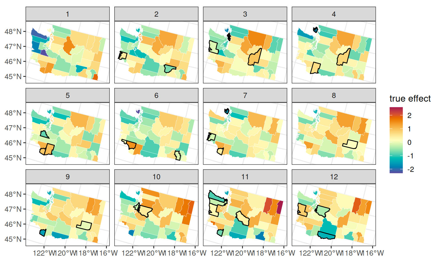
5 Fit
Rows with y = NA are included in the fitting data so the held-out county-time nodes remain in the latent support. They do not contribute to the observed likelihood, but they can be recovered and predicted after fitting.
The process term has one variance parameter, one spatial CAR association parameter rho, and one temporal AR(1) parameter phi.
Code
stLMM summary
  formula: y ~ x + car_time(area, time, graph = g)
  observations: 468 (438 observed, 30 missing response)
  posterior draws: 500
  family: gaussian
  fixed effects: 2
  grouped random-effect coefficients: 0
  process terms: 1
  residual variance: global tau_sq

beta:
               mean     sd    q2.5   q50.0   q97.5
(Intercept)  0.6297 0.1175  0.4104  0.6267  0.8624
x           -0.7679 0.1228 -1.0160 -0.7669 -0.5320

tau_sq:
       mean     sd  q2.5  q50.0  q97.5
value 0.009 0.0079 4e-04 0.0073 0.0297

sigma_sq:
                      mean     sd   q2.5  q50.0  q97.5
car_time_1_sigma_sq 2.0563 0.2294 1.6443 2.0597 2.6599

theta:
                 mean     sd   q2.5  q50.0  q97.5
car_time_1_rho 0.6277 0.0915 0.4373 0.6349 0.7775
car_time_1_phi 0.7916 0.0237 0.7414 0.7920 0.8378
6 Recover
The CAR-time latent process is integrated out during fitting. Calling recover() draws the county-time effects conditional on posterior parameter samples.
stLMM recovery
  formula: y ~ x + car_time(area, time, graph = g)
  observations: 468 (438 observed, 30 missing response)
  recovered draws: 151
  recovered process terms: car_time_1
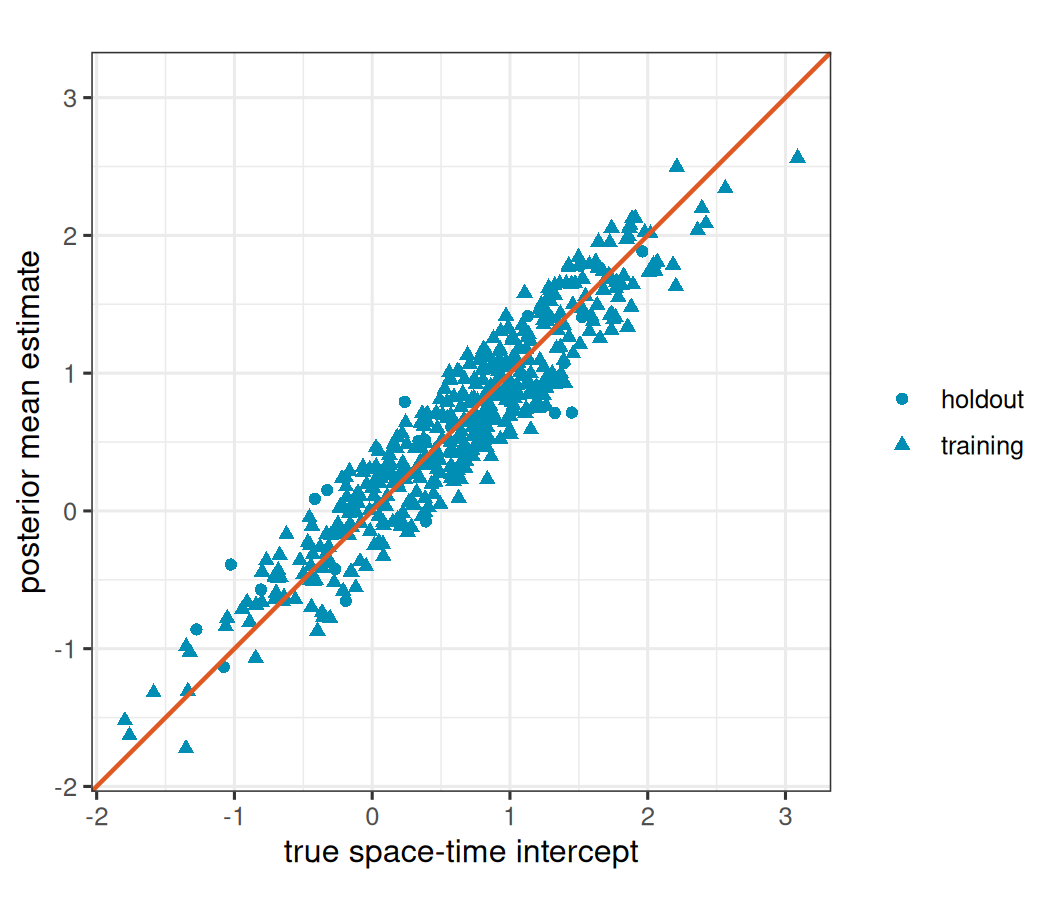
As in the areal CAR vignette, the data identify the combined space-time intercept, \(\beta_0 + w_{it}\), more directly than the split between the global intercept and the average level of one realized process. For this diagnostic, we compare \(\beta_0 + w_{it}\) rather than \(w_{it}\) alone.
Show plotting code
rec_draws <- as_samples(rec, include_w = TRUE, metadata = FALSE)
w_cols <- paste0("w_car_time_1_", seq_len(nrow(dat)))
w_hat <- colMeans(rec_draws[, w_cols, drop = FALSE])
beta_0_hat <- mean(rec_draws[["(Intercept)"]])

recovery_dat <- data.frame(
  truth = beta[1] + dat$w_true,
  estimate = beta_0_hat + w_hat,
  sample = dat$sample
)
recovery_lim <- range(recovery_dat$truth, recovery_dat$estimate)

ggplot(recovery_dat, aes(truth, estimate)) +
  geom_point(
    aes(shape = sample),
    color = stlmm_color("primary"),
    size = 1.8
  ) +
  geom_abline(
    intercept = 0,
    slope = 1,
    color = stlmm_color("secondary"),
    linewidth = 0.8
  ) +
  coord_equal(
    xlim = recovery_lim,
    ylim = recovery_lim
  ) +
  labs(
    x = "true space-time intercept",
    y = "posterior mean estimate",
    shape = NULL
  )
7 Predict
CAR-time prediction is limited to area-time combinations that already belong to the fitted graph and time support. Here the held-out observations meet that condition because their rows were included in the original data with y = NA.
Code
stLMM prediction
  mean samples: 151 draws x 30 rows
  newdata: TRUE
  joint: FALSE
  y samples: simulated
  process samples: car_time_1
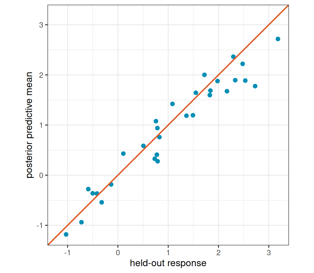
The predict() call returns posterior draws of \(\mu\) in mu_samples and, because y_samples = TRUE, posterior predictive response draws in y_samples. Printing the prediction object gives a compact overview; summary(pred) gives posterior summaries for these draws.
Show plotting code
pred_y <- as_samples(pred, sample = "y", metadata = FALSE)
pred_dat <- data.frame(
  y = dat$y_full[holdout_id],
  y_hat = colMeans(pred_y)
)
pred_lim <- range(pred_dat$y, pred_dat$y_hat)

ggplot(pred_dat, aes(y, y_hat)) +
  geom_point(
    color = stlmm_color("primary"),
    size = 2
  ) +
  geom_abline(
    intercept = 0,
    slope = 1,
    color = stlmm_color("secondary"),
    linewidth = 0.8
  ) +
  coord_equal(
    xlim = pred_lim,
    ylim = pred_lim
  ) +
  labs(
    x = "held-out response",
    y = "posterior predictive mean"
  )
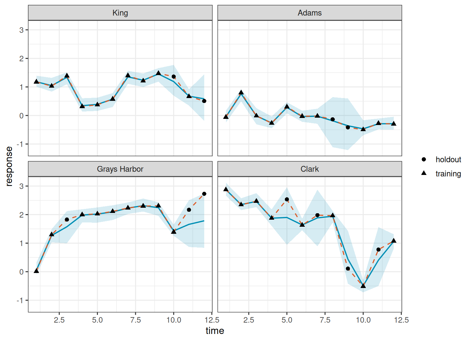
To see how prediction uncertainty changes over time, it is useful to look at complete county time series and mark the missing response times. First, predict across the full fitted support.
Code
pred_all <- predict(
  rec,
  y_samples = TRUE
)
Below, the shaded bands are pointwise 95% posterior predictive intervals. The intervals are often wider at held-out times because those rows are informed by neighboring counties, adjacent times, and the fitted mean structure, but not by their own observed response.
Show plotting code
series_dat <- dat
pred_all_y <- as_samples(pred_all, sample = "y", metadata = FALSE)
series_dat$y_mean <- colMeans(pred_all_y)
series_dat$y_lower <- NA_real_
series_dat$y_upper <- NA_real_
for(j in seq_len(ncol(pred_all_y))){
  q <- quantile(pred_all_y[, j], probs = c(0.025, 0.975))
  series_dat$y_lower[j] <- q[1]
  series_dat$y_upper[j] <- q[2]
}

area_count <- data.frame(area = unique(dat$area), holdout = 0)
for(j in seq_len(nrow(area_count))){
  area_count$holdout[j] <- sum(dat$area[holdout_id] == area_count$area[j])
}
area_count <- area_count[order(-area_count$holdout), ]
series_area <- head(area_count$area, 4)
series_dat <- series_dat[series_dat$area %in% series_area, ]
series_dat$county <- factor(series_dat$county, levels = unique(series_dat$county))

ggplot(series_dat, aes(time)) +
  geom_ribbon(
    aes(ymin = y_lower, ymax = y_upper),
    fill = stlmm_color("primary"),
    alpha = 0.16
  ) +
  geom_line(
    aes(y = y_mean),
    color = stlmm_color("primary"),
    linewidth = 0.7
  ) +
  geom_line(
    aes(y = y_full),
    color = stlmm_color("secondary"),
    linewidth = 0.6,
    linetype = "dashed"
  ) +
  geom_point(
    aes(y = y_full, shape = sample),
    size = 2
  ) +
  facet_wrap(~ county, ncol = 2) +
  labs(
    x = "time",
    y = "response",
    shape = NULL
  )
8 Exponential time option
The AR(1) time model treats the sorted time support as a lattice. If the time values are numeric and the gaps themselves should matter, use time_model = "exp" as follows.
With time_model = "exp", the temporal correlation is \(\exp\{-\lambda |t-t'|\}\) and the fitted time values must be numeric. This is also the covariance function of a continuous-time Ornstein-Uhlenbeck (OU) process. For observations on a one-dimensional ordered time axis, the inverse correlation matrix is sparse and tridiagonal, even when the time gaps are unequal. This is why time_model = "exp" still works naturally with the sparse precision calculations used by car_time(). For this simulated example, we would expect similar results from the two time models. The AR(1) and exponential-time models are closely related: an OU process observed at equally spaced times has AR(1)-type correlation, and the simulated time values used above are equally spaced.
9 What this example illustrates
The car_time() term is useful when the same areal units are observed repeatedly over time and the random effects should be smooth across both neighboring areas and nearby times. In this example, counties define the areal support and the time column defines the temporal support. Rows with y = NA let us hold out county-time responses while still keeping those county-time random effects available for recovery and prediction.
The default AR(1) time model is a good choice when the fitted time values are treated as ordered steps. The exponential time option is available when the actual numeric time gaps should matter.