
Point observations with areal space-time effects
Plot-level rows mapped to county-year CAR-time support
Source:vignettes/a04-point-observations-car-time.qmd
1 Overview
This vignette shows how point-referenced observations can be modeled with an areal space-time latent process. This setting is common when observations arise at points, but the usable spatial identifier is coarser than the true point location. For example, exact coordinates may be unavailable, intentionally coarsened, or withheld for confidentiality, while the areal unit and time associated with each observation remain available for analysis.
In reality, point responses often arise from a finer-scale spatial or space-time process. An CAR-time effect should therefore be interpreted as a latent effect on the available areal support, not as a claim that the true fine-scale process is constant within each area-time. For this vignette, we simulate from the model we fit so the indexing, recovery, and prediction behavior can be checked directly.
2 Model
Let \(k\) index point-referenced observations. Each observation belongs to area \(a(k)\) and time \(t(k)\). The model is
\[ y_k = \beta_0 + x_k\beta_1 + w_{a(k),t(k)} + \epsilon_k,\qquad \epsilon_k \sim N(0,\tau^2). \]
The latent process \(w_{a,t}\) is a separable CAR-time process over areas and times. Multiple point observations can map to the same area-time latent node, and some area-time nodes can have no point observations. The model is similar to the space-time CAR model in the previous vignette, but the response rows are point-referenced observations rather than area-time observations.
3 County graph
We again use Washington counties from stunitco with the island bridge rule.
Code
   from    to  distance
1 53055 53029  56295.36
2 53055 53035 100454.10
3 53055 53073 100817.65
4 53055 53057 102288.17
The graph object stores binary adjacency and any bridge edges added by the island rule. In this vignette, the graph defines the county support for the CAR-time random effects; the point coordinates are used only to show where the simulated observations fall.
4 Simulated County-Year Effects
We first simulate the county-year latent effects on the full areal space-time support. The CAR-time dependence is parameterized through the separable precision matrix \(\mathbf{Q}\). However, in the simulation code below, rmvnorm() draws from a covariance matrix, so we compute \(\mathbf{\Sigma} = \mathbf{Q}^{-1}\) before drawing the county-year effects.
Code
year <- 1:12

centroid_x <- sf::st_coordinates(sf::st_centroid(sf::st_geometry(wa_counties)))[, "X"]
centroid_x_mean <- mean(centroid_x)
centroid_x_sd <- stats::sd(centroid_x)

county_dat <- data.frame(
  area = as.character(wa_counties$COUNTYFIPS),
  county = wa_counties$COUNTYNM,
  x = (centroid_x - centroid_x_mean) / centroid_x_sd
)

support <- expand.grid(
  year = year,
  area = county_dat$area
)
support <- support[order(support$area, support$year), ]
support$county <- county_dat$county[match(support$area, county_dat$area)]
support$x <- county_dat$x[match(support$area, county_dat$area)]

beta <- c(0.5, 1)
sigma_sq <- 1
rho <- 0.5
phi <- 0.75
tau_sq <- 0.01

Q_space <- car_prec(g, sigma_sq = 1, rho = rho)
Q_time <- ar1_prec(year, sigma_sq = 1, phi = phi)
Q <- (1 / sigma_sq) * kronecker(Q_space, Q_time)
Sigma <- solve(Q)

support$w_true <- rmvnorm(mean = rep(0, nrow(Q)), Sigma = Sigma)
The support object is the full latent county-year support. expand.grid() creates one row for every combination of year and county, the rows are sorted to match the internal car_time() ordering, and the county covariate is then copied onto each county-year row. This ordering is only needed for the manual simulation step. In the stLMM() call, the package builds the latent CAR-time support internally from the graph IDs and the specified time column, so the input rows don’t need to be sorted this way.
The observed point data below will cover only part of this support. For car_time(), county-years with no point observations are still available for recovery and prediction as long as the county is in the graph and the year appears somewhere in the fitting data. If an entire year has no observations, add a row with y = NA and the associated year, area, and covariate values to include that year in the fitted time support.
5 Point Observations
Next we sample 20 counties in each year and generate one to four point observations within each sampled county-year. Counties not sampled in a given year have no point observations for that year, but they remain part of the latent CAR-time support. The point coordinates are used only to visualize the simulated sampling pattern. The fitted model below uses county and year, not point coordinates.
Code
n_county_per_year <- 20
sampled_nodes <- data.frame()

for(yy in year){
  year_nodes <- support[support$year == yy, ]
  sampled_county <- sample(seq_len(nrow(year_nodes)), n_county_per_year)
  sampled_nodes <- rbind(sampled_nodes, year_nodes[sampled_county, ])
}

sampled_nodes$n_plot <- sample(1:4, nrow(sampled_nodes), replace = TRUE)

plot_dat <- sampled_nodes[rep(seq_len(nrow(sampled_nodes)), sampled_nodes$n_plot), ]
rownames(plot_dat) <- NULL

plot_dat$x <- plot_dat$x + rnorm(nrow(plot_dat), sd = 0.5)
mu <- beta[1] + beta[2] * plot_dat$x + plot_dat$w_true
epsilon <- rnorm(nrow(plot_dat), sd = sqrt(tau_sq))
plot_dat$y <- mu + epsilon

point_coord <- matrix(NA, nrow(plot_dat), 2)
for(i in seq_len(nrow(county_dat))){
  point_id <- which(plot_dat$area == county_dat$area[i])
  if(length(point_id) > 0){
    point_geom <- sf::st_sample(wa_counties[i, ], size = length(point_id))
    point_coord[point_id, ] <- sf::st_coordinates(point_geom)[, 1:2, drop = FALSE]
  }
}

plot_dat$X <- point_coord[, 1]
plot_dat$Y <- point_coord[, 2]
The faceted map shows the simulated point observations. Some county-years have several points, while others have none. The fitted model uses the area and year columns to connect each point observation to its county-year random effect.
Show plotting code
point_sf <- sf::st_as_sf(
  plot_dat,
  coords = c("X", "Y"),
  crs = sf::st_crs(wa_counties)
)

ggplot() +
  geom_sf(
    data = wa_counties,
    fill = "grey95",
    color = "white",
    linewidth = 0.1
  ) +
  geom_sf(
    data = point_sf,
    aes(color = y),
    size = 0.8,
    alpha = 0.75
  ) +
  scale_color_gradientn(colors = stlmm_palette()) +
  facet_wrap(~ year, ncol = 4) +
  labs(color = "response")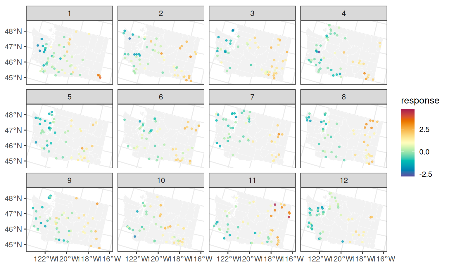
6 Fit
The formula uses the point-level covariate x, but the latent process term uses only area and year. The warning about duplicated area-time values is expected because multiple point observations can map to the same county-year latent node. The residual and process variances use half-\(t\) priors on their corresponding standard deviations. The spatial CAR association parameter rho and temporal AR(1) parameter phi use bounded uniform priors.
Code
Warning: duplicated area-time values detected in car_time(area, year); fitting
latent process on 468 area-time nodes (from 612 observations)
Code
summary(fit)stLMM summary
formula: y ~ x + car_time(area, year, graph = g)
observations: 612
posterior draws: 400
family: gaussian
fixed effects: 2
grouped random-effect coefficients: 0
process terms: 1
residual variance: global tau_sq
beta:
mean sd q2.5 q50.0 q97.5
(Intercept) 0.5722 0.1081 0.3800 0.5657 0.8077
x 1.0099 0.0135 0.9874 1.0087 1.0383
tau_sq:
mean sd q2.5 q50.0 q97.5
value 0.0146 0.0225 0.0086 0.0112 0.0636
sigma_sq:
mean sd q2.5 q50.0 q97.5
car_time_1_sigma_sq 0.8439 0.1516 0.5911 0.8554 1.1135
theta:
mean sd q2.5 q50.0 q97.5
car_time_1_rho 0.8363 0.0729 0.6651 0.8708 0.9031
car_time_1_phi 0.6470 0.2417 0.0124 0.7485 0.82347 Recover county-year effects
The CAR-time latent process is integrated out during fitting. Calling recover() draws the county-year effects on the full county-year support, including county-year nodes without point observations.
stLMM recovery
  formula: y ~ x + car_time(area, year, graph = g)
  observations: 612
  recovered draws: 126
  recovered process terms: car_time_1
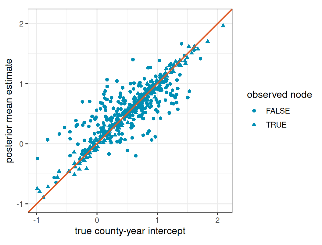
As in the previous CAR vignettes, the data identify the combined county-year intercept, \(\beta_0 + w_{a,t}\), more directly than the split between the global intercept and the average level of one realized process. For this diagnostic, we compare \(\beta_0 + w_{a,t}\) rather than \(w_{a,t}\) alone.
Show plotting code
rec_draws <- as_samples(rec, include_w = TRUE, metadata = FALSE)
w_cols <- paste0("w_car_time_1_", seq_len(nrow(support)))
w_hat <- colMeans(rec_draws[, w_cols, drop = FALSE])
beta_0_hat <- mean(rec_draws[["(Intercept)"]])

support$observed <- FALSE
for(j in seq_len(nrow(support))){
  support$observed[j] <- any(
    plot_dat$area == support$area[j] &
      plot_dat$year == support$year[j]
  )
}

recovery_dat <- data.frame(
  truth = beta[1] + support$w_true,
  estimate = beta_0_hat + w_hat,
  observed = support$observed
)
recovery_lim <- range(recovery_dat$truth, recovery_dat$estimate)

ggplot(recovery_dat, aes(truth, estimate)) +
  geom_point(
    aes(shape = observed),
    color = stlmm_color("primary"),
    size = 1.7
  ) +
  geom_abline(
    intercept = 0,
    slope = 1,
    color = stlmm_color("secondary"),
    linewidth = 0.8
  ) +
  coord_equal(
    xlim = recovery_lim,
    ylim = recovery_lim
  ) +
  labs(
    x = "true county-year intercept",
    y = "posterior mean estimate",
    shape = "observed node"
  )
8 Predict county-year means
For a county-year summary, create a prediction grid with one row per county-year. Here we use the county covariate value as the prediction covariate. The predict() call returns posterior draws of \(\mu\) in mu_samples and, because y_samples = TRUE, posterior predictive response draws in y_samples.
Code
stLMM prediction
  mean samples: 126 draws x 468 rows
  newdata: TRUE
  joint: FALSE
  y samples: simulated
  process samples: car_time_1
The faceted map summarizes posterior predictive response means for every county-year in the fitted support. County-years with no point observations are outlined in black.
Show plotting code
pred_y <- as_samples(pred, sample = "y", metadata = FALSE)
pred_grid$y_hat <- colMeans(pred_y)
pred_grid$observed <- FALSE
for(j in seq_len(nrow(pred_grid))){
  pred_grid$observed[j] <- any(
    plot_dat$area == pred_grid$area[j] &
      plot_dat$year == pred_grid$year[j]
  )
}

pred_map <- merge(
  wa_counties,
  pred_grid,
  by.x = "COUNTYFIPS",
  by.y = "area"
)

ggplot(pred_map) +
  geom_sf(
    aes(fill = y_hat),
    color = "white",
    linewidth = 0.1
  ) +
  geom_sf(
    data = pred_map[!pred_map$observed, ],
    fill = NA,
    color = "black",
    linewidth = 0.35
  ) +
  scale_fill_gradientn(colors = stlmm_palette()) +
  facet_wrap(~ year, ncol = 4) +
  labs(fill = "predicted")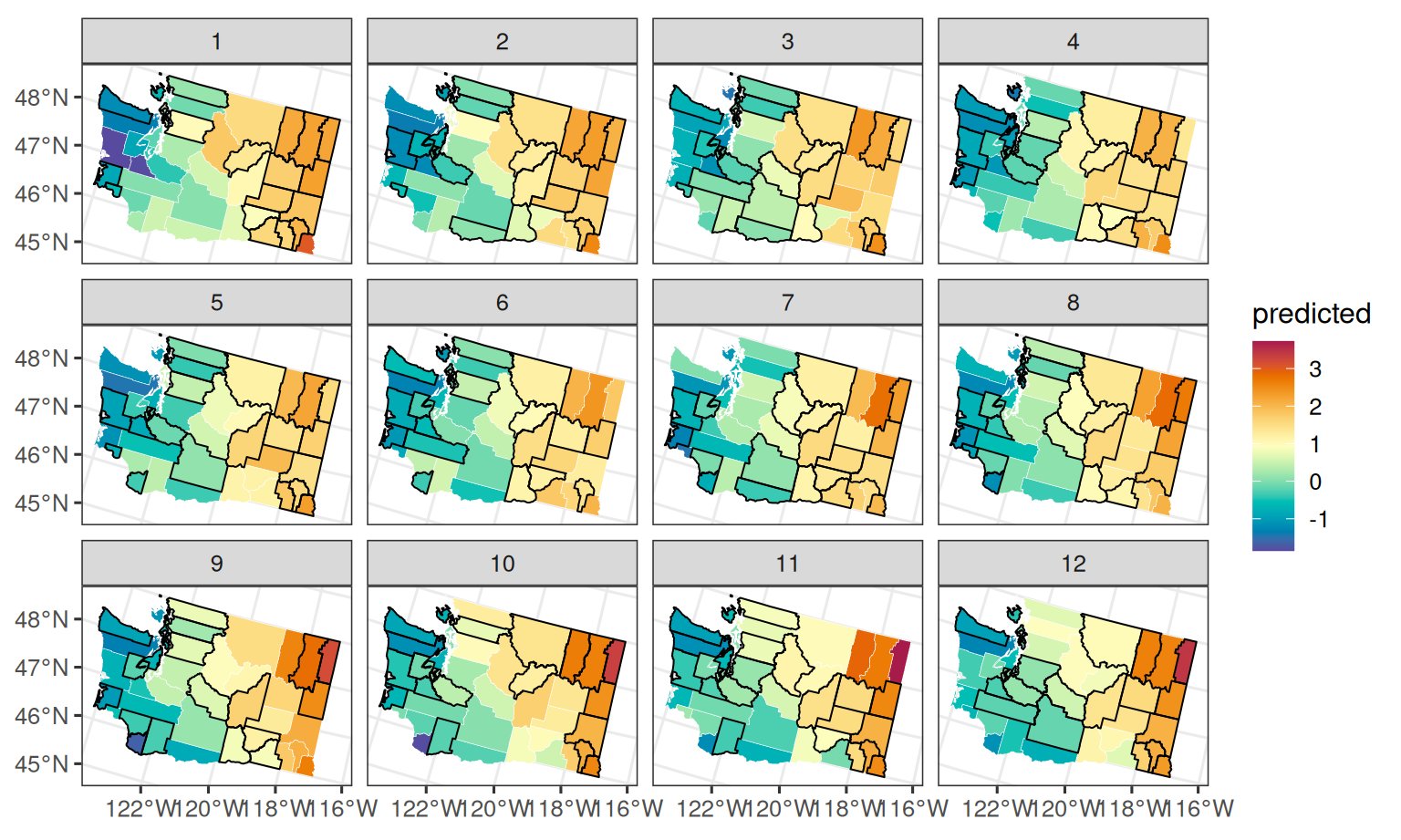
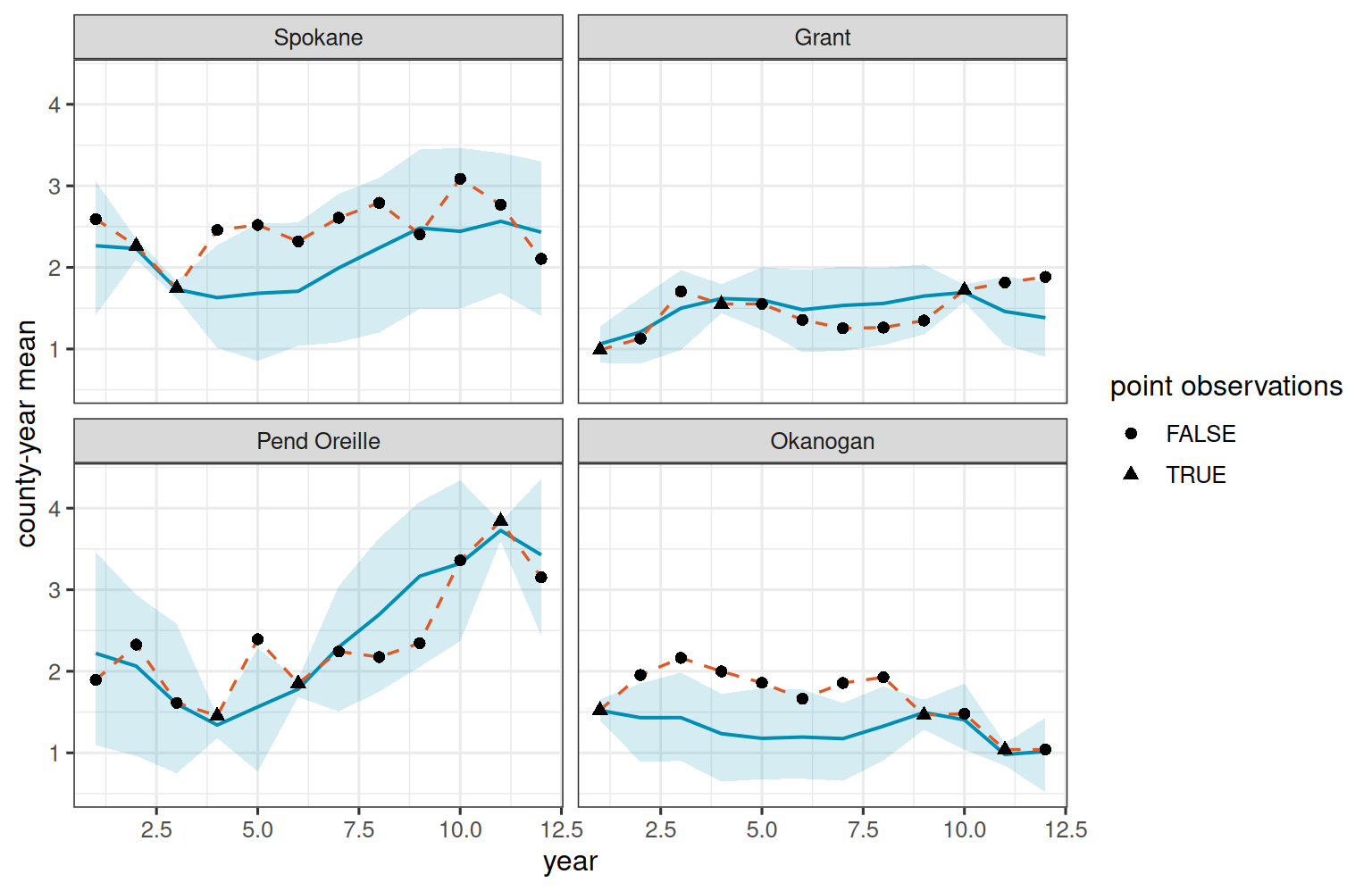
The map is useful for checking spatial patterns, but county profiles make the temporal behavior easier to see. Below we select four counties with several unobserved county-years. The shaded bands are pointwise 95% posterior intervals for \(\mu\), the solid line is the posterior mean, and the dashed line is the true county-year mean used in the simulation. The points mark whether each county-year had any point observations.
Show plotting code
profile_dat <- pred_grid
pred_mu <- as_samples(pred, sample = "mu", metadata = FALSE)
profile_dat$mu_mean <- colMeans(pred_mu)
profile_dat$mu_lower <- NA_real_
profile_dat$mu_upper <- NA_real_
for(j in seq_len(ncol(pred_mu))){
  q <- quantile(pred_mu[, j], probs = c(0.025, 0.975))
  profile_dat$mu_lower[j] <- q[1]
  profile_dat$mu_upper[j] <- q[2]
}
profile_dat$true_mean <- beta[1] + beta[2] * profile_dat$x + support$w_true

area_count <- data.frame(area = unique(profile_dat$area), unobserved = 0)
for(j in seq_len(nrow(area_count))){
  area_count$unobserved[j] <- sum(!profile_dat$observed[profile_dat$area == area_count$area[j]])
}
area_count <- area_count[order(-area_count$unobserved), ]
profile_area <- head(area_count$area, 4)
profile_dat <- profile_dat[profile_dat$area %in% profile_area, ]
profile_dat$county <- factor(profile_dat$county, levels = unique(profile_dat$county))

ggplot(profile_dat, aes(year)) +
  geom_ribbon(
    aes(ymin = mu_lower, ymax = mu_upper),
    fill = stlmm_color("primary"),
    alpha = 0.16
  ) +
  geom_line(
    aes(y = mu_mean),
    color = stlmm_color("primary"),
    linewidth = 0.7
  ) +
  geom_line(
    aes(y = true_mean),
    color = stlmm_color("secondary"),
    linewidth = 0.6,
    linetype = "dashed"
  ) +
  geom_point(
    aes(y = true_mean, shape = observed),
    size = 2
  ) +
  facet_wrap(~ county, ncol = 2) +
  labs(
    x = "year",
    y = "county-year mean",
    shape = "point observations"
  )
9 What this example illustrates
The data rows don’t have to be one row per latent process node. Here many point observations map to the same county-year effect, and many county-year effects have no point observations. The fitted car_time() model uses the available county-year support to share information across neighboring counties and adjacent years, while the point-level covariate and residual variance remain observation-level quantities.
The example uses the default ordered-support AR(1) time model. If the time values are numeric and the gaps themselves should matter, use car_time(area, year, graph = g, time_model = "exp"). With time_model = "exp", the temporal correlation is \(\exp\{-\lambda |t-t'|\}\) and the fitted time values must be numeric.