
Spatially varying coefficients with stLMM
Covariate-scaled NNGP terms, recovery, and prediction
Source:vignettes/a06-spatial-varying-coefficients.qmd
1 Overview
Any structured process term in stLMM can be used as a covariate-scaled random effect. The formula syntax follows the usual interaction form. For example, x:nngp(lon, lat) gives a spatially varying coefficient for x, x:ar1(day) gives a time-varying coefficient, and x:car(area, graph = g) gives an areal spatially varying coefficient.
This vignette demonstrates the idea with an NNGP spatially varying coefficient. We simulate repeated observations at spatial locations, fit an NNGP model with both a spatially varying intercept and a spatially varying slope, recover the fitted coefficient surfaces, and predict held-out observations. The repeated observations are useful here because they give the model information to separate the local intercept from the local slope.
2 Model
For observation \(j\) at location \(\mathbf{s}_i = (s_{i1}, s_{i2})^\top\), the model is
\[ y_{ij} = \beta_0 + w_0(\mathbf{s}_i) + x_{ij}\{\beta_1 + w_1(\mathbf{s}_i)\} + \epsilon_{ij},\qquad \epsilon_{ij} \sim N(0,\tau^2). \]
The two spatial processes are independent:
\[ \mathbf{w}_0 \sim N(\mathbf{0}, \sigma_0^2 \mathbf{R}_0(\phi_0)), \qquad \mathbf{w}_1 \sim N(\mathbf{0}, \sigma_1^2 \mathbf{R}_1(\phi_1)), \]
with exponential correlation functions
\[ R_{k,ij}(\phi_k) = \exp\{-\phi_k \|\mathbf{s}_i - \mathbf{s}_j\|\}, \qquad k = 0, 1. \]
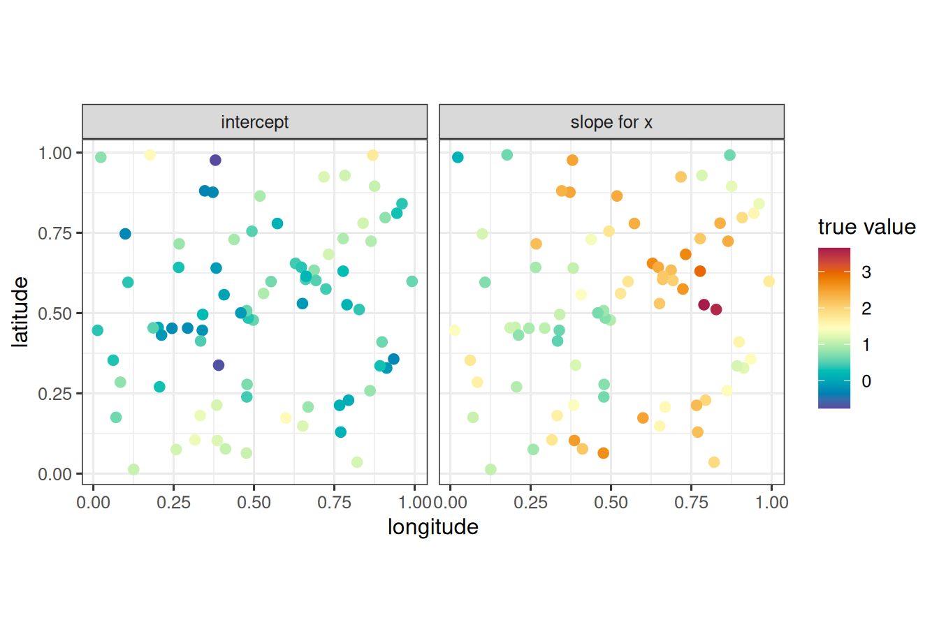
The first process, \(w_0(\mathbf{s})\), makes the intercept vary over space. The second process, \(w_1(\mathbf{s})\), makes the coefficient for \(x\) vary over space. The coefficient surface for \(x\) is therefore \(\beta_1 + w_1(\mathbf{s})\), not \(w_1(\mathbf{s})\) alone.
3 Data
We simulate locations in the unit square. At each location, we generate three observations with different values of x. The full Gaussian process covariance is used to simulate the two spatial surfaces. The fitted model uses nngp() as a nearest-neighbor approximation to the full process, as in the spatial NNGP vignette.
Code
n_train_node <- 80
n_holdout_node <- 12
n_rep <- 3
n_node <- n_train_node + n_holdout_node

coords <- data.frame(
  lon = runif(n_node),
  lat = runif(n_node)
)

node <- rep(seq_len(n_node), each = n_rep)
dat <- data.frame(
  node = node,
  lon = coords$lon[node],
  lat = coords$lat[node]
)

dat$x <- rep(c(-1, 0, 1), times = n_node) + rnorm(n_node * n_rep, sd = 0.05)

beta <- c(0.7, 1.2)
tau_sq <- 0.05

sigma_sq_intercept <- 0.45
phi_intercept <- 5
sigma_sq_slope <- 0.45
phi_slope <- 4

C_intercept <- exp_cov(
  coords = coords,
  sigma_sq = sigma_sq_intercept,
  phi = phi_intercept
)
C_slope <- exp_cov(
  coords = coords,
  sigma_sq = sigma_sq_slope,
  phi = phi_slope
)

w_intercept <- rmvnorm(mean = rep(0, n_node), Sigma = C_intercept)
w_slope <- rmvnorm(mean = rep(0, n_node), Sigma = C_slope)

dat$intercept_true <- beta[1] + w_intercept[node]
dat$slope_true <- beta[2] + w_slope[node]
dat$mu <- dat$intercept_true + dat$x * dat$slope_true
dat$y <- dat$mu + rnorm(nrow(dat), sd = sqrt(tau_sq))

train <- dat[dat$node <= n_train_node, ]
holdout <- dat[dat$node > n_train_node, ]
Show plotting code
plot_nodes <- data.frame(
  lon = coords$lon[seq_len(n_train_node)],
  lat = coords$lat[seq_len(n_train_node)],
  intercept = beta[1] + w_intercept[seq_len(n_train_node)],
  slope = beta[2] + w_slope[seq_len(n_train_node)]
)

plot_dat <- rbind(
  data.frame(
    lon = plot_nodes$lon,
    lat = plot_nodes$lat,
    surface = "intercept",
    value = plot_nodes$intercept
  ),
  data.frame(
    lon = plot_nodes$lon,
    lat = plot_nodes$lat,
    surface = "slope for x",
    value = plot_nodes$slope
  )
)

ggplot(plot_dat, aes(lon, lat)) +
  geom_point(
    aes(color = value),
    size = 2.2
  ) +
  facet_wrap(~ surface) +
  scale_color_gradientn(colors = stlmm_palette()) +
  coord_equal() +
  labs(
    x = "longitude",
    y = "latitude",
    color = "true value"
  )
4 Fit
The model formula includes x as a fixed effect and then adds two structured process terms. The first nngp(lon, lat, ...) term is the spatially varying intercept. The second term, x:nngp(lon, lat, ...), is the spatially varying coefficient for x.
The two NNGP terms use separate covariance parameters. In the fitted object, the intercept process is named nngp_1 and the spatially varying coefficient process is named nngp_2.
Code
fit <- stLMM(
  y ~ x +
    nngp(lon, lat, m = 15, cov_model = "exp", ordering = "maxmin") +
    x:nngp(lon, lat, m = 15, cov_model = "exp", ordering = "maxmin"),
  data = train,
  priors = list(
    resid = list(tau_sq = half_t(df = 3, scale = 0.3)),
    nngp_1 = list(
      sigma_sq = half_t(df = 3, scale = 0.8),
      phi = uniform(1, 20)
    ),
    nngp_2 = list(
      sigma_sq = half_t(df = 3, scale = 0.8),
      phi = uniform(1, 20)
    )
  ),
  n_samples = 1500,
  verbose = FALSE
)

summary(fit)
stLMM summary
formula: y ~ x + nngp(lon, lat, m = 15, cov_model = "exp", ordering = "maxmin") + x:nngp(lon, lat, m = 15, cov_model = "exp", ordering = "maxmin")
observations: 240
posterior draws: 1500
family: gaussian
fixed effects: 2
grouped random-effect coefficients: 0
process terms: 2
residual variance: global tau_sq
beta:
mean sd q2.5 q50.0 q97.5
(Intercept) 0.5948 0.1751 0.2739 0.5857 0.9603
x 1.4447 0.3501 0.6879 1.4589 2.0685
tau_sq:
mean sd q2.5 q50.0 q97.5
value 0.0616 0.0097 0.0458 0.0605 0.0841
sigma_sq:
mean sd q2.5 q50.0 q97.5
nngp_1_sigma_sq 0.3707 0.0952 0.2205 0.3578 0.6081
nngp_2_sigma_sq 0.6340 0.2115 0.3582 0.5748 1.2055
theta:
mean sd q2.5 q50.0 q97.5
nngp_1_phi 8.9662 3.1626 4.1373 8.3641 17.2337
nngp_2_phi 4.2473 1.5416 1.9871 3.8720 7.74005 Recover
Structured process terms are integrated out during fitting. Calling recover() draws the fitted spatial process values conditional on the retained posterior samples.
stLMM recovery
  formula: y ~ x + nngp(lon, lat, m = 15, cov_model = "exp", ordering = "maxmin") + x:nngp(lon, lat, m = 15, cov_model = "exp", ordering = "maxmin")
  observations: 240
  recovered draws: 500
  recovered process terms: nngp_1, nngp_2
For direct coda workflows, as_mcmc(rec, include_w = TRUE) returns the fixed-effect, covariance-parameter, and recovered coefficient-process samples aligned to the recovered posterior iterations. The plotting code below uses as_samples() because data-frame columns are easier to manipulate when separating intercept and slope surfaces.
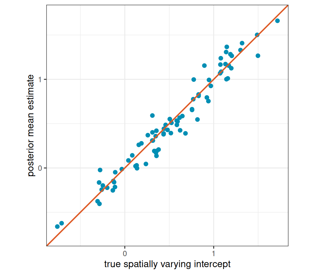
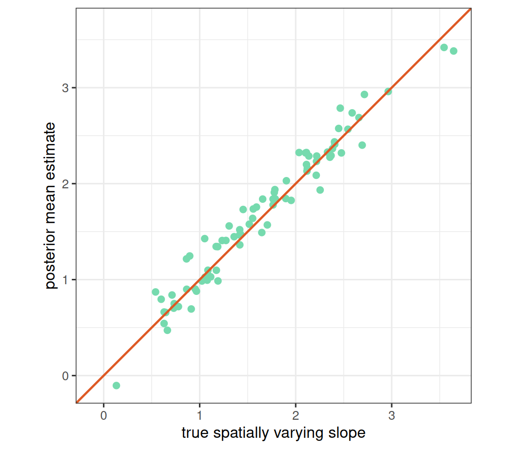
The recovered nngp_1 values are the spatial intercept deviations \(w_0(\mathbf{s}_i)\). The recovered nngp_2 values are the spatial slope deviations \(w_1(\mathbf{s}_i)\). To compare with the simulated coefficient surfaces, add the corresponding fixed-effect posterior mean.
Because the data have repeated observations at each training location, the recovered NNGP columns correspond to the unique training locations. We simulated and sorted the training data by node, so those columns align with coords[1:n_train_node, ].
Show plotting code
intercept_lim <- range(recovery_dat$true_intercept, recovery_dat$estimated_intercept)

ggplot(recovery_dat, aes(true_intercept, estimated_intercept)) +
  geom_point(
    color = stlmm_color("primary"),
    size = 2
  ) +
  geom_abline(
    intercept = 0,
    slope = 1,
    color = stlmm_color("secondary"),
    linewidth = 0.8
  ) +
  coord_equal(
    xlim = intercept_lim,
    ylim = intercept_lim
  ) +
  labs(
    x = "true spatially varying intercept",
    y = "posterior mean estimate"
  )
Show plotting code
slope_lim <- range(recovery_dat$true_slope, recovery_dat$estimated_slope)

ggplot(recovery_dat, aes(true_slope, estimated_slope)) +
  geom_point(
    color = stlmm_color("accent"),
    size = 2
  ) +
  geom_abline(
    intercept = 0,
    slope = 1,
    color = stlmm_color("secondary"),
    linewidth = 0.8
  ) +
  coord_equal(
    xlim = slope_lim,
    ylim = slope_lim
  ) +
  labs(
    x = "true spatially varying slope",
    y = "posterior mean estimate"
  )
6 Predict
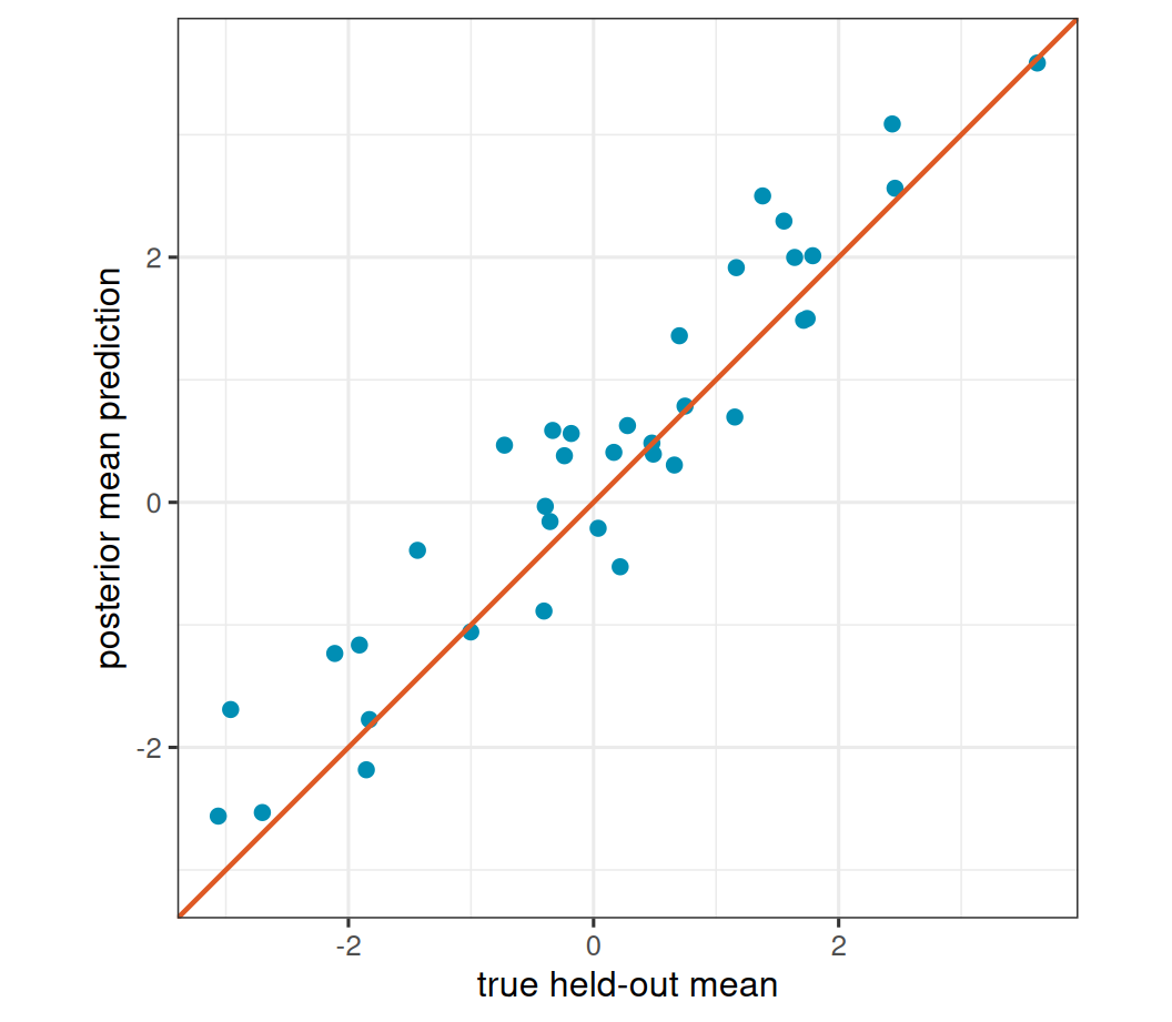
Prediction works the same way as in the spatial NNGP vignette, except the new data must include the covariate used in the spatially varying coefficient term. The predicted mean combines the fixed effects, the predicted intercept process, and the predicted slope process multiplied by the new x value.
Code
stLMM prediction
  mean samples: 500 draws x 36 rows
  newdata: TRUE
  joint: FALSE
  y samples: simulated
  process samples: nngp_1, nngp_2
When return_w_samples = TRUE, the retained process samples include the raw predicted slope deviations \(w_1(\mathbf{s})\). They do not include the covariate scaling. The scaling by x is applied when constructing the predicted means.
Show plotting code
pred_draws <- as_samples(pred, sample = "all", metadata = FALSE)
mu_cols <- paste0("mu_", seq_len(nrow(holdout_new)))
y_cols <- paste0("y_", seq_len(nrow(holdout_new)))
pred_dat <- data.frame(
  mu = holdout$mu,
  mu_hat = colMeans(pred_draws[, mu_cols, drop = FALSE]),
  y = holdout$y,
  y_hat = colMeans(pred_draws[, y_cols, drop = FALSE])
)

pred_lim <- range(pred_dat$mu, pred_dat$mu_hat)

ggplot(pred_dat, aes(mu, mu_hat)) +
  geom_point(
    color = stlmm_color("primary"),
    size = 2
  ) +
  geom_abline(
    intercept = 0,
    slope = 1,
    color = stlmm_color("secondary"),
    linewidth = 0.8
  ) +
  coord_equal(
    xlim = pred_lim,
    ylim = pred_lim
  ) +
  labs(
    x = "true held-out mean",
    y = "posterior mean prediction"
  )
7 What this example illustrates
The formula x:nngp(lon, lat) does not add another fixed effect for x; it adds a spatial process whose contribution is multiplied by x. Including both x and x:nngp(lon, lat) gives a global average slope plus a spatial deviation from that slope.
The same pattern applies to other structured terms. A covariate can scale an ar1() term for a time-varying coefficient, a car() term for an areal spatially varying coefficient, or a car_time() term for a space-time varying coefficient. The interpretation is the same: recover the raw latent process, then add the corresponding fixed effect when you want the full coefficient surface.
8 Graphs and Sparse Factorization
One useful design detail is visible if we ask stLMM to print its term description before sampling. Setting describe_terms = TRUE prints the fixed-effect structure, process terms, graph indices, sparse matrix size, and CHOLMOD factorization diagnostics. The same option can be used with the model above; the example below uses fewer retained samples only to keep the vignette quick.
Code
fit_described <- stLMM(
  y ~ x +
    nngp(lon, lat, m = 15, cov_model = "exp", ordering = "maxmin") +
    x:nngp(lon, lat, m = 15, cov_model = "exp", ordering = "maxmin"),
  data = train,
  priors = list(
    resid = list(tau_sq = half_t(df = 3, scale = 0.3)),
    nngp_1 = list(
      sigma_sq = half_t(df = 3, scale = 0.8),
      phi = uniform(1, 20)
    ),
    nngp_2 = list(
      sigma_sq = half_t(df = 3, scale = 0.8),
      phi = uniform(1, 20)
    )
  ),
  n_samples = 5,
  describe_terms = TRUE,
  verbose = FALSE
)
========================================================================
stLMM term description
========================================================================
Model summary
------------------------------------------------------------------------
formula: y ~ x + nngp(lon, lat, m = 15, cov_model = "exp", ordering = "maxmin") + x:nngp(lon, lat, m = 15, cov_model = "exp", ordering = "maxmin")
n: 240
p: 2
q: 0
qLatTotal: 160
process terms: 2
explicit random-effect terms: 0
graphs: 1
M dimensions: 160 x 160
M nnz: 3260
CHOLMOD ordering: amd
CHOLMOD fill ratio: 2.332
CHOLMOD lnz: 7602
CHOLMOD flops: 465530
factorization status: success
Fixed effects (X)
------------------------------------------------------------------------
columns (p): 2
names: (Intercept), x
Explicit random effects (Z)
------------------------------------------------------------------------
none
Process terms
------------------------------------------------------------------------
[1] nngp_1
label: nngp(lon, lat, m = 15, cov_model = "exp", ordering = "maxmin")
type: nngp
graph index: 1
covariance model: exp
SVC term: no
n linked observations: 240
latent nodes: 80
q_lat: 80
w_offset: 1
repeated indices collapsed: yes
unique locations: 80
sigma^2 current: 1
sigma^2 tuning: 0.1
sigma^2 prior: inverse-gamma(shape=2, scale=1)
theta parameters:
- phi: current=10.5, tuning=0.1, bounds=(1, 20), prior=uniform, transform=bounded-logit
coord dimension: 2
neighbor count m: 15
ordering: maxmin
repeated coordinates collapsed: yes
neighbor summary: min=0.000, mean=13.500, max=15.000
prior precision nnz: 1590
------------------------------------------------------------------------
[2] nngp_2
label: x:nngp(lon, lat, m = 15, cov_model = "exp", ordering = "maxmin")
type: nngp
graph index: 1
covariance model: exp
SVC term: yes
n linked observations: 240
latent nodes: 80
q_lat: 80
w_offset: 81
repeated indices collapsed: yes
unique locations: 80
sigma^2 current: 1
sigma^2 tuning: 0.1
sigma^2 prior: inverse-gamma(shape=2, scale=1)
theta parameters:
- phi: current=10.5, tuning=0.1, bounds=(1, 20), prior=uniform, transform=bounded-logit
coord dimension: 2
neighbor count m: 15
ordering: maxmin
repeated coordinates collapsed: yes
neighbor summary: min=0.000, mean=13.500, max=15.000
prior precision nnz: 1590
========================================================================The output shows two process terms but only one graph. The first process term, nngp_1, is the spatially varying intercept and is not an SVC term. The second process term, nngp_2, is the x:nngp(...) term and is marked as an SVC term. Both terms have graph index: 1, which means they reuse the same NNGP graph: the same spatial support, neighbor count, ordering, and neighbor pattern. They still have separate covariance parameters and separate latent process values. Reusing the graph avoids rebuilding an identical nearest-neighbor structure for each term.
The model summary also reports the sparse matrix used by the collapsed sampler. Here M dimensions is the dimension of the latent sparse matrix \(\mathbf{M}\), and M nnz is the number of stored nonzero entries in its sparse pattern. NNGP terms are useful computationally because each node is connected only to a small neighbor set, so the prior precision contribution is sparse.
After the sparse pattern is built, stLMM uses CHOLMOD, a sparse Cholesky factorization library for sparse symmetric positive definite matrices (Chen et al. 2008), through the R Matrix package’s sparse matrix interface (Bates et al. 2025). CHOLMOD performs a symbolic analysis of the sparsity pattern and chooses a fill-reducing ordering; in this run the reported ordering is amd, approximate minimum degree. This ordering is internal to the factorization. It does not change the spatial coordinates, the NNGP neighbor graph, or the statistical model. Its job is to reduce fill-in, meaning new nonzero entries created in the Cholesky factor that were not present in the original sparse matrix pattern. If CHOLMOD is compiled with METIS support, it can also use graph-partitioning orderings based on multilevel partitioning ideas (Karypis and Kumar 1998), which can reduce fill-in and factorization work for some sparse matrix patterns. Once the symbolic structure is available, later numerical factorizations can reuse that structure as covariance and variance parameters change.
The remaining CHOLMOD diagnostics are computational, not statistical. CHOLMOD fill ratio compares the size of the factor pattern to the original sparse matrix pattern. CHOLMOD lnz reports the number of nonzero entries in the Cholesky factor, and CHOLMOD flops reports the approximate floating-point work for the factorization. These quantities help explain why graph structure, repeated-location collapsing, shared graph reuse, and the NNGP neighbor count m can matter for runtime.
This sparse-matrix view is central to the package design. NNGP, CAR, and autoregressive terms all produce sparse precision matrices, and stLMM is built around using that sparsity with CHOLMOD sparse factorization rather than treating the latent process covariance as dense. The lower-level dense linear algebra used inside these routines is handled by BLAS and LAPACK (Blackford et al. 2002; Anderson et al. 1999). Because those libraries are supplied by the user’s R installation, the same package code can benefit from optimized or threaded BLAS/LAPACK implementations when R is linked against them. One common open-source choice is OpenBLAS (OpenBLAS Project 2025), though the best option depends on the user’s operating system, processor, and R installation. For a deeper look at CHOLMOD ordering, fill-in diagnostics, OpenMP threads, BLAS/LAPACK choices, and reproducible timing scripts, see the runtime-performance article.