
Residual variance options with stLMM
From constant variance to heteroskedastic and direct-estimate models
Source:vignettes/a07-residual-variance-options.qmd
1 Overview
This vignette introduces residual variance options in Gaussian models. We start with the constant residual variance model used in earlier vignettes, then generalize to group-specific residual variances for grouped heteroskedasticity. The final examples move to a small-area estimation setting where the response is a direct estimate and the dataset includes externally supplied sampling variance estimates.
2 Constant residual variance
The default Gaussian residual model estimates a single residual variance
\[ y_i = \beta_0 + x_i\beta_1 + \epsilon_i,\qquad \epsilon_i \sim N(0,\tau^2). \]
This is the residual model used in the earlier introductory examples. The simulation builds the mean theta, then adds independent Gaussian residual error.
Code
n <- 80

constant_dat <- data.frame(
  x = runif(n, -1, 1)
)

beta <- c(0.5, 1)
tau_sq <- 0.25^2

mu <- beta[1] + beta[2] * constant_dat$x
epsilon <- rnorm(n, sd = sqrt(tau_sq))

constant_dat$theta <- mu
constant_dat$y <- mu + epsilon
Show plotting code
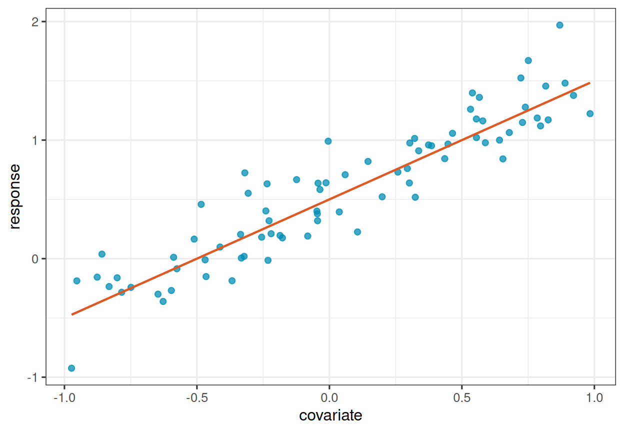
Code
stLMM summary
  formula: y ~ x
  observations: 80
  posterior draws: 400
  family: gaussian
  fixed effects: 2
  grouped random-effect coefficients: 0
  process terms: 0
  residual variance: global tau_sq

beta:
              mean     sd   q2.5  q50.0  q97.5
(Intercept) 0.5275 0.0263 0.4765 0.5269 0.5793
x           1.0041 0.0490 0.9030 1.0052 1.0976

tau_sq:
        mean   sd   q2.5  q50.0  q97.5
value 0.0503 0.01 0.0331 0.0497 0.0691
Recall that the prior is associated with the variance parameter tau_sq, but half_t(df = 3, scale = 0.5) is placed on the residual standard deviation, \(\tau = \sqrt{\tau^2}\), and transformed internally to the variance scale.
3 Group-specific residual variances
A common generalization is to let the residual variance differ by group. The grouping variable could indicate sampling strata, measurement protocols, ownership classes, forest types, or any other known classification where residual variation is expected to differ.
\[ y_i = \beta_0 + x_i\beta_1 + \epsilon_i,\qquad \epsilon_i \sim N(0,\tau_{g_i}^2). \]
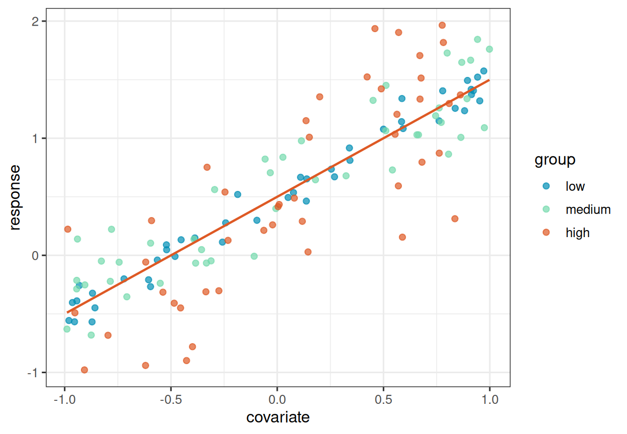
The simulated dataset has three groups with the same mean model and different residual standard deviations.
Code
n_group <- 3
n_per_group <- 45
group_name <- c("low", "medium", "high")
group_sd <- c(low = 0.10, medium = 0.25, high = 0.50)

group_dat <- data.frame(
  group = factor(rep(group_name, each = n_per_group), levels = group_name),
  x = runif(n_group * n_per_group, -1, 1)
)

beta <- c(0.5, 1)
mu <- beta[1] + beta[2] * group_dat$x

group_dat$theta <- mu
group_dat$tau_sq_true <- group_sd[as.character(group_dat$group)]^2
group_dat$y <- mu + rnorm(nrow(group_dat), sd = sqrt(group_dat$tau_sq_true))
Show plotting code
ggplot(group_dat, aes(x, y)) +
  geom_point(
    aes(color = group),
    alpha = 0.7,
    size = 1.8
  ) +
  geom_line(
    aes(y = theta),
    color = stlmm_color("secondary"),
    linewidth = 0.8
  ) +
  scale_color_manual(
    values = stlmm_discrete_colors(3)
  ) +
  labs(
    x = "covariate",
    y = "response",
    color = "group"
  )
For comparison, first fit the constant residual variance model to the grouped data.
Code
stLMM summary
  formula: y ~ x
  observations: 135
  posterior draws: 400
  family: gaussian
  fixed effects: 2
  grouped random-effect coefficients: 0
  process terms: 0
  residual variance: global tau_sq

beta:
              mean     sd   q2.5  q50.0  q97.5
(Intercept) 0.4994 0.0283 0.4466 0.4993 0.5519
x           1.0410 0.0479 0.9517 1.0413 1.1307

tau_sq:
       mean    sd   q2.5  q50.0  q97.5
value 0.123 0.015 0.0959 0.1216 0.1558
Now fit the group-specific residual variance model. A single prior can be recycled over all groups using priors$resid, or group-specific priors can be supplied with names matching the observed groups. Here we use one weakly informative half-\(t\) prior for all three residual standard deviations.
Code
stLMM summary
  formula: y ~ x + resid(model = "group", group = group)
  observations: 135
  posterior draws: 500
  family: gaussian
  fixed effects: 2
  grouped random-effect coefficients: 0
  process terms: 0
  residual variance: sampled group-specific values

beta:
              mean     sd   q2.5  q50.0  q97.5
(Intercept) 0.5019 0.0149 0.4719 0.5016 0.5296
x           1.0092 0.0214 0.9657 1.0093 1.0495

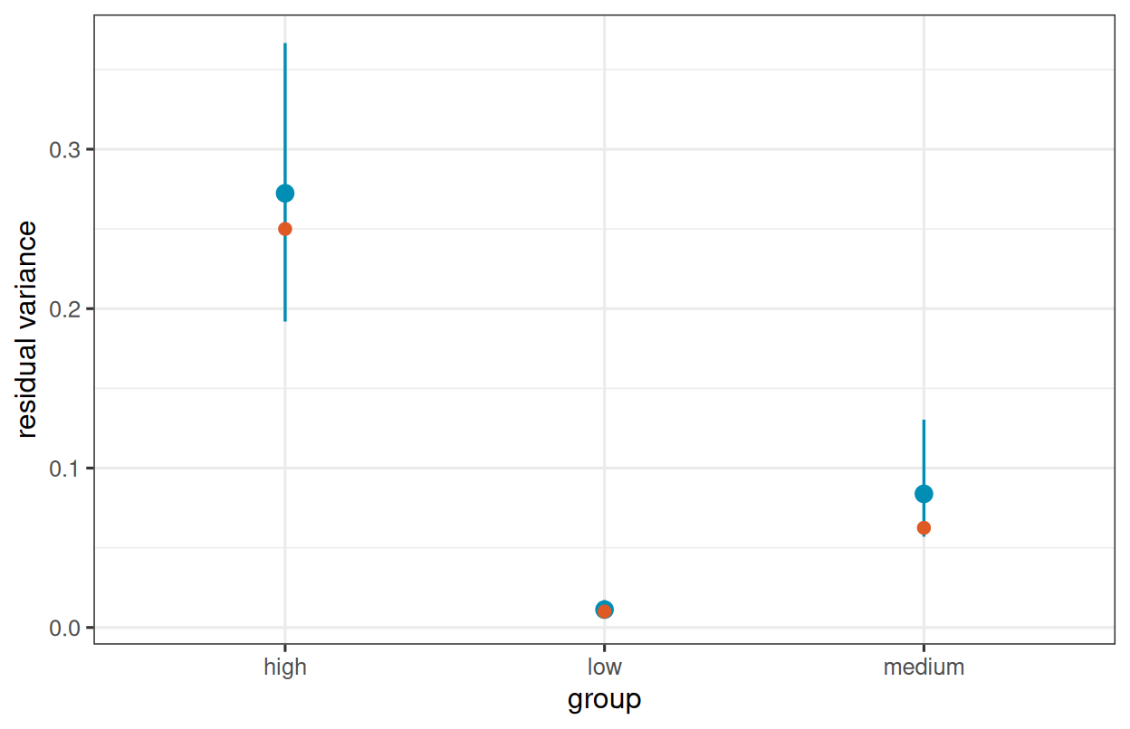
residual_variance:
                mean     sd   q2.5  q50.0  q97.5
tau_sq_low    0.0112 0.0024 0.0072 0.0109 0.0172
tau_sq_medium 0.0838 0.0194 0.0569 0.0806 0.1304
tau_sq_high   0.2724 0.0472 0.1919 0.2675 0.3666
Code
variance_cols <- paste0("tau_sq_", group_name)
variance_draws <- as_samples(fit_group_variance, metadata = FALSE)[, variance_cols, drop = FALSE]
group_variance_summary <- data.frame(
  group = group_name,
  truth = group_sd[group_name]^2,
  posterior_mean = colMeans(variance_draws),
  posterior_lower = NA_real_,
  posterior_upper = NA_real_
)

for(j in seq_len(nrow(group_variance_summary))){
  q <- quantile(
    variance_draws[, j],
    probs = c(0.025, 0.975)
  )
  group_variance_summary$posterior_lower[j] <- q[1]
  group_variance_summary$posterior_upper[j] <- q[2]
}

group_variance_summary
group truth posterior_mean posterior_lower posterior_upper
low low 0.0100 0.01123045 0.007211225 0.01717942
medium medium 0.0625 0.08382252 0.056940692 0.13039497
high high 0.2500 0.27235880 0.191889784 0.36658595Show plotting code
ggplot(group_variance_summary, aes(group, posterior_mean)) +
  geom_pointrange(
    aes(ymin = posterior_lower, ymax = posterior_upper),
    color = stlmm_color("primary"),
    linewidth = 0.6
  ) +
  geom_point(
    aes(y = truth),
    color = stlmm_color("secondary"),
    size = 2
  ) +
  labs(
    x = "group",
    y = "residual variance"
  )
4 Direct-estimate setting
Suppose area \(i\) has a direct estimate \(\hat{y}_i\) for an underlying area-level target \(\theta_i\). A simple working model is
\[ \hat{y}_i = \theta_i + e_i,\qquad e_i \sim N(0, v_i), \]
where \(v_i\) is the direct-estimate sampling variance. The mean model is
\[ \theta_i = \beta_0 + x_i\beta_1. \]
In many small-area applications, \(v_i\) is supplied by a design-based estimator or another external procedure. The residual variance model controls how that variance information enters stLMM. The simulation below makes direct estimates more precise when the effective sample size is larger.
Code
n_area <- 100

direct_dat <- data.frame(
  area = sprintf("area_%02d", seq_len(n_area)),
  x = runif(n_area, -1, 1),
  n_eff = sample(10:100, n_area, replace = TRUE)
)

beta <- c(0.5, 1)
mu <- beta[1] + beta[2] * direct_dat$x
direct_dat$theta <- mu

reference_se <- 0.5
reference_n <- 30

direct_dat$vhat <- reference_se^2 * reference_n / direct_dat$n_eff

direct_dat$yhat <- mu + rnorm(n_area, sd = sqrt(direct_dat$vhat))
Show plotting code
ggplot(direct_dat, aes(x, yhat)) +
  geom_point(
    aes(size = 1 / vhat),
    color = stlmm_color("primary"),
    alpha = 0.7
  ) +
  geom_line(
    aes(y = theta),
    color = stlmm_color("secondary"),
    linewidth = 0.8
  ) +
  scale_size_continuous(
    range = c(1.5, 4)
  ) +
  labs(
    x = "area covariate",
    y = "direct estimate",
    size = "precision"
  )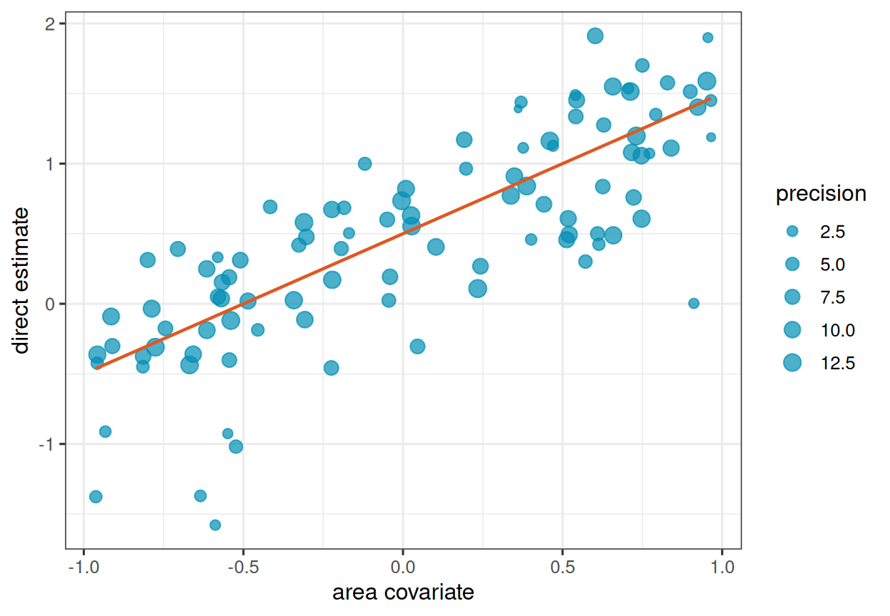
The plot shows the direct estimates around the latent area-level mean. Point size is proportional to the supplied direct-estimate precision, \(1/v_i\). Larger points have smaller supplied sampling variances and therefore carry more information about the corresponding latent area mean.
4.1 Fixed direct-estimate variances
When the direct-estimate variances are treated as known sampling variances, use resid(model = "fixed", variance = vhat). In this model, tau_sq is not estimated; instead, the observation-level precision is fixed at \(1/v_i\).
Code
stLMM summary
  formula: yhat ~ x + resid(model = "fixed", variance = vhat)
  observations: 100
  posterior draws: 400
  family: gaussian
  fixed effects: 2
  grouped random-effect coefficients: 0
  process terms: 0
  residual variance: fixed row-specific values

beta:
              mean     sd  q2.5  q50.0  q97.5
(Intercept) 0.4724 0.0377 0.395 0.4746 0.5349
x           0.9203 0.0581 0.808 0.9214 1.0323
The fitted object reports that fixed row-specific residual variances are being used. Because tau_sq is replaced by the supplied vhat column, no tau_sq prior is included.
4.2 Fay-Herriot models
The fixed direct-estimate variance model above is the sampling model used in Fay-Herriot small-area models (Fay and Herriot 1979). A basic Fay-Herriot model adds an area-level random effect to the latent mean
\[ \hat{\theta}_i = \theta_i + e_i,\qquad e_i \sim N(0, v_i), \]
\[ \theta_i = \mathbf{x}_i^\top\mathbf{\beta} + \alpha_i,\qquad \alpha_i \sim N(0,\sigma_\alpha^2). \]
In stLMM, the sampling model is specified with resid(model = "fixed", variance = vhat), and the independent area effects are specified with iid(area).
Code
stLMM fit
  formula: yhat ~ x + iid(area) + resid(model = "fixed", variance = vhat)
  observations: 100
  family: gaussian
  posterior draws: 400
  fixed effects: 2
  grouped random-effect coefficients: 100
  process terms: 0
  residual variance: fixed row-specific values
  samples: beta, alpha, iid_sigma_sq
  sampler elapsed: 0.064 seconds
Here the response rows are area-level direct estimates. The iid(area) term is the Fay-Herriot area random effect: it models residual variation in the latent area means \(\theta_i\) after accounting for the covariate. The direct-estimate sampling variances enter separately through resid(model = "fixed", variance = vhat).
4.3 Prior-informed sampling variances
The classical Fay-Herriot model treats \(v_i\) as known. In practice, direct-estimate variances are often estimated from the same sparse survey data that produce the direct estimates. Shannon et al. (2025) motivate using the direct variance estimate and effective sample size to define an inverse-gamma prior for the sampling-error variance rather than fixing it.
In stLMM, resid(model = "group", group = area, variance = vhat, prior = "ig") estimates one sampling-error variance per group and uses vhat to construct its prior. With this prior, the same inverse-gamma shape is used for every group. If center = "mode", the supplied vhat_g is the most likely prior value for the group-specific sampling variance \(\tau_g^2\):
\[ \tau_g^2 \sim IG(a, b_g),\qquad b_g = (a + 1)\hat{v}_g. \]
The shape value \(a\) controls how strongly the prior is concentrated around vhat_g. Smaller values allow the sampled variance to move farther from vhat_g; larger values place more prior mass near vhat_g. This is useful when vhat_g is informative but should not be treated as exact.
Code
stLMM fit
  formula: yhat ~ x + iid(area) + resid(model = "group", group = area, variance = vhat, prior = "ig", shape = 10, center = "mode")
  observations: 100
  family: gaussian
  posterior draws: 400
  fixed effects: 2
  grouped random-effect coefficients: 100
  process terms: 0
  residual variance: sampled group-specific values
  samples: beta, alpha, residual_variance, iid_sigma_sq
  sampler elapsed: 0.082 seconds
This model keeps the Fay-Herriot sampling and linking structure, but the observation variance is sampled. The supplied vhat anchors the prior for each area-level sampling-error variance. The Shannon construction is also available with method = "shannon", which sets the inverse-gamma shape and scale from both vhat and n_eff.
5 Spatial Fay-Herriot models
A spatial Fay-Herriot model keeps the same direct-estimate sampling model but replaces the independent area effects with spatially structured area effects. With a CAR model,
\[ \theta_i = \mathbf{x}_i^\top\mathbf{\beta} + w_i,\qquad \mathbf{w} \sim N(\mathbf{0}, \mathbf{Q}_{\mathrm{car}}^{-1}). \]
We use Washington counties to simulate a spatial Fay-Herriot example. The county graph is the same graph construction used in the areal CAR vignette.
Code
data(stunitco, package = "stLMM")

wa_counties <- stunitco[stunitco$STATECD == 53, ]
g <- car_graph(wa_counties, id = "COUNTYFIPS", island = "nearest")

centroid_x <- sf::st_coordinates(sf::st_centroid(sf::st_geometry(wa_counties)))[, "X"]
centroid_x_mean <- mean(centroid_x)
centroid_x_sd <- stats::sd(centroid_x)

wa_dat <- data.frame(
  area = as.character(wa_counties$COUNTYFIPS),
  county = wa_counties$COUNTYNM,
  x = (centroid_x - centroid_x_mean) / centroid_x_sd,
  n_eff = sample(10:100, nrow(wa_counties), replace = TRUE)
)

beta_wa <- c(0.5, -1)
sigma_sq_wa <- 0.25
rho_wa <- 0.75

Q_wa <- car_prec(g, sigma_sq = sigma_sq_wa, rho = rho_wa)
w_wa <- rmvnorm(mean = rep(0, nrow(Q_wa)), Sigma = solve(Q_wa))
names(w_wa) <- rownames(Q_wa)

wa_dat$w_true <- w_wa[wa_dat$area]
mu <- beta_wa[1] + beta_wa[2] * wa_dat$x + wa_dat$w_true
wa_dat$theta <- mu
wa_reference_se <- 0.25
wa_reference_n <- 30

wa_dat$vhat <- wa_reference_se^2 * wa_reference_n / wa_dat$n_eff
wa_dat$yhat <- mu + rnorm(nrow(wa_dat), sd = sqrt(wa_dat$vhat))
Show plotting code
wa_plot <- wa_counties
wa_plot$area <- as.character(wa_plot$COUNTYFIPS)
wa_plot$theta <- wa_dat$theta[match(wa_plot$area, wa_dat$area)]
wa_plot$yhat <- wa_dat$yhat[match(wa_plot$area, wa_dat$area)]

wa_map <- rbind(
  transform(wa_plot, value = theta, quantity = "latent area mean"),
  transform(wa_plot, value = yhat, quantity = "direct estimate")
)

ggplot(wa_map) +
  geom_sf(
    aes(fill = value),
    color = "white",
    linewidth = 0.15
  ) +
  facet_wrap(~ quantity) +
  scale_fill_gradientn(colors = stlmm_palette()) +
  labs(
    fill = "value"
  )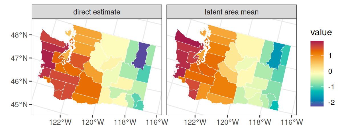
The direct estimates are noisier than the latent area means, especially for counties with smaller effective sample sizes. Because the simulation treats vhat as the data-generating sampling variance, the spatial Fay-Herriot fit below uses resid(model = "fixed", variance = vhat). The model uses the supplied sampling variances and county graph to smooth the direct estimates.
Code
stLMM fit
  formula: yhat ~ x + car(area, graph = g) + resid(model = "fixed", variance = vhat)
  observations: 39
  family: gaussian
  posterior draws: 500
  fixed effects: 2
  grouped random-effect coefficients: 0
  process terms: 1
  residual variance: fixed row-specific values
  samples: beta, sigma_sq, theta
  latent process samples: not retained; call recover()
  sampler elapsed: 0.02 seconds
This example shows the spatial Fay-Herriot workflow and the role of the residual variance model. With one simulated areal field over 39 counties, the CAR variance and dependence parameters can be weakly identified. Longer runs, stronger prior information, repeated time points, or more areas are needed before interpreting the covariance parameter estimates closely.
Code
spatial_fh_recovery <- recover(fit_spatial_fh)
wa_dat$fitted_mean <- fitted(spatial_fh_recovery)

direct_rmse <- sqrt(mean((wa_dat$yhat - wa_dat$theta)^2))
fitted_rmse <- sqrt(mean((wa_dat$fitted_mean - wa_dat$theta)^2))

spatial_fh_summary <- data.frame(
  quantity = c("direct estimate", "spatial FH fitted"),
  rmse = c(direct_rmse, fitted_rmse)
)

spatial_fh_summary
quantity rmse
1 direct estimate 0.2551759
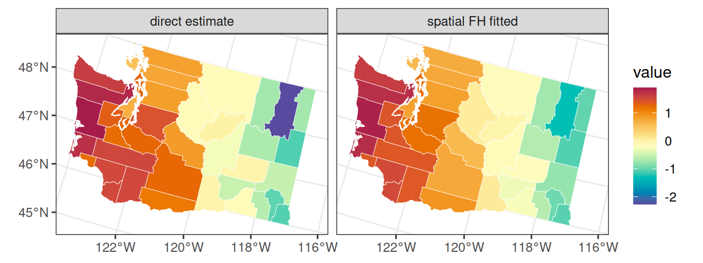
2 spatial FH fitted 0.1984263In this simulation, the spatial Fay-Herriot fitted means have a smaller RMSE than the direct estimates. The improvement is modest, which is what we should expect from a small example: the direct estimates already contain useful information, and the spatial model mainly borrows strength from neighboring counties while accounting for the supplied sampling-variance information.
Show plotting code
wa_plot$fitted_mean <- wa_dat$fitted_mean[match(wa_plot$area, wa_dat$area)]

wa_fit_map <- rbind(
  transform(wa_plot, value = yhat, quantity = "direct estimate"),
  transform(wa_plot, value = fitted_mean, quantity = "spatial FH fitted")
)

ggplot(wa_fit_map) +
  geom_sf(
    aes(fill = value),
    color = "white",
    linewidth = 0.15
  ) +
  facet_wrap(~ quantity) +
  scale_fill_gradientn(colors = stlmm_palette()) +
  labs(
    fill = "value"
  )
6 What this example illustrates
The default Gaussian residual model estimates one tau_sq. Use resid(model = "group", group = group) when residual variance is expected to differ across a modest number of groups. This is a heteroskedastic residual model, not a direct-estimate row-specific variance model. Use priors$resid to give one prior for all group-specific residual variances or a named prior for each group.
Use resid(model = "fixed", variance = vhat) when row-specific variances are treated as known sampling variances for direct estimates. Use resid(model = "group", group = area, variance = vhat, prior = "ig", shape = ..., center = ...) when direct variance estimates should anchor, rather than fix, sampled observation variances. With center = "mode", vhat is the most likely prior value and shape controls concentration. Use resid(model = "group", group = area, variance = vhat, n = n_eff, prior = "shannon") when an effective sample size should determine the inverse-gamma prior shape and scale. Adding iid(area) gives a basic Fay-Herriot model with independent area effects. Replacing iid(area) with car(area, graph) gives a spatial Fay-Herriot-style model that borrows strength across neighboring areas.
Prediction with y_samples = TRUE requires the corresponding residual variance information in newdata, such as vhat, n_eff, or group. Models with many sampled residual variance groups can mix slowly because those variance parameters are part of the Metropolis updates.