Negative-binomial count models with stLMM

Fixed-size NB-PG likelihoods with areal CAR effects

Andrew O. Finley

Show preliminaries

library(stLMM)
library(ggplot2)
library(sf)

source(file.path(dirname(knitr::current_input(dir = TRUE)), "utils.R"))

set.seed(14)

1 Overview

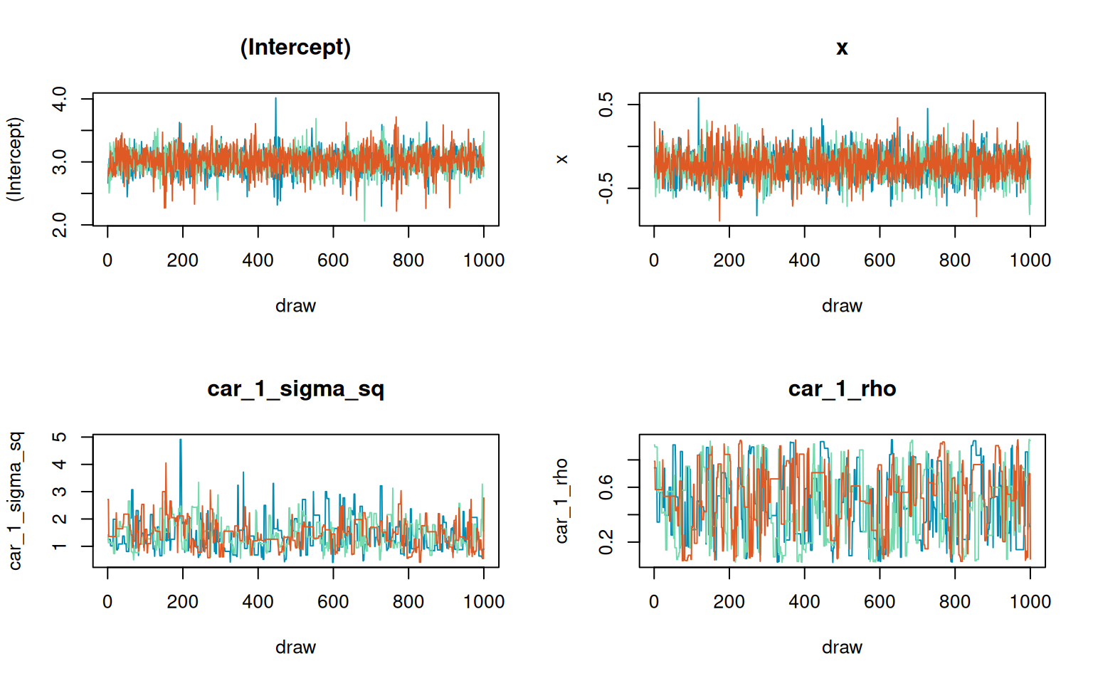
This vignette introduces count models in stLMM using family = "negative_binomial". The example uses the bundled stunitco county polygon layer, extracts Washington counties, builds a county adjacency graph, simulates areal counts with a CAR latent effect and a known exposure offset, and fits fixed-size negative-binomial models using Pólya-Gamma updates. The fits use three chains so the trace plots can be inspected directly.

There are two simulation sections. The first generates counts from a negative-binomial model with known size and fits the same likelihood. The second generates Poisson counts and fits a large-size negative-binomial model to show how the fixed-size NB likelihood can approximate a Poisson log-mean model. The examples avoid extremely sparse counts, because very sparse count data provide little information about a latent areal surface.

2 Count model

For area \(i\), stLMM uses the negative-binomial mean parameterization

\[ y_i \mid \mu_i, r \sim \operatorname{NB}(r, \mu_i), \qquad E(y_i) = \mu_i, \qquad \operatorname{var}(y_i) = \mu_i + \frac{\mu_i^2}{r}, \]

where \(r\) is the fixed size argument. The log mean is modeled as

\[ \eta_i = \log(\mu_i) = o_i + \beta_0 + x_i\beta_1 + w_i. \]

Here \(o_i\) is a known formula offset. In the simulations below, \(o_i = \log(e_i)\) for a known exposure multiplier \(e_i\).

Internally, the Pólya-Gamma augmentation uses the logit probability tilt

\[ \psi_i = \eta_i - \log(r), \]

and draws

\[ \omega_i \mid \psi_i, y_i, r \sim \operatorname{PG}(y_i + r, \psi_i). \]

Conditional on \(\omega_i\), the likelihood is Gaussian in \(\eta_i\) with working response

\[ z_i = \frac{(y_i-r)/2}{\omega_i} + \log(r). \]

This is the same Pólya-Gamma identity used for binomial logistic regression, applied to the negative-binomial logit-probability representation (Polson et al. 2013; Windle et al. 2013). The package uses this conditionally Gaussian form to reuse the sparse collapsed sampler used by the Gaussian and binomial models.

The size parameter is fixed in this implementation. A larger size reduces overdispersion and moves the negative-binomial distribution toward a Poisson distribution. Extremely large size values are not always better computationally because the Pólya-Gamma shape is \(y_i + r\).

3 County graph

We use the same Washington county graph as the areal CAR vignette. The graph defines the latent areal support and the neighbor relationships used by car().

Code

data(stunitco, package = "stLMM")

wa_counties <- stunitco[stunitco$STATECD == 53, ]
g <- car_graph(wa_counties, id = "COUNTYFIPS", island = "nearest", island_k = 4)

Show edge-map code

coord_dat <- data.frame(
  area = as.character(wa_counties$COUNTYFIPS),
  sf::st_coordinates(
    sf::st_point_on_surface(sf::st_geometry(wa_counties))
  )
)

edge_index <- which(as.matrix(g$adjacency) != 0, arr.ind = TRUE)
edge_index <- edge_index[edge_index[, "row"] < edge_index[, "col"], , drop = FALSE]
edge_dat <- data.frame(
  from = g$ids[edge_index[, "row"]],
  to = g$ids[edge_index[, "col"]]
)
edge_dat$x <- coord_dat$X[match(edge_dat$from, coord_dat$area)]
edge_dat$y <- coord_dat$Y[match(edge_dat$from, coord_dat$area)]
edge_dat$xend <- coord_dat$X[match(edge_dat$to, coord_dat$area)]
edge_dat$yend <- coord_dat$Y[match(edge_dat$to, coord_dat$area)]

ggplot(wa_counties) +
  geom_sf(fill = "grey95", color = "white", linewidth = 0.15) +
  geom_segment(
    data = edge_dat,
    aes(x = x, y = y, xend = xend, yend = yend),
    color = "grey45",
    linewidth = 0.25
  ) +
  geom_point(
    data = coord_dat,
    aes(X, Y),
    color = stlmm_color("primary"),
    size = 1.4
  ) +
  labs(x = "longitude", y = "latitude")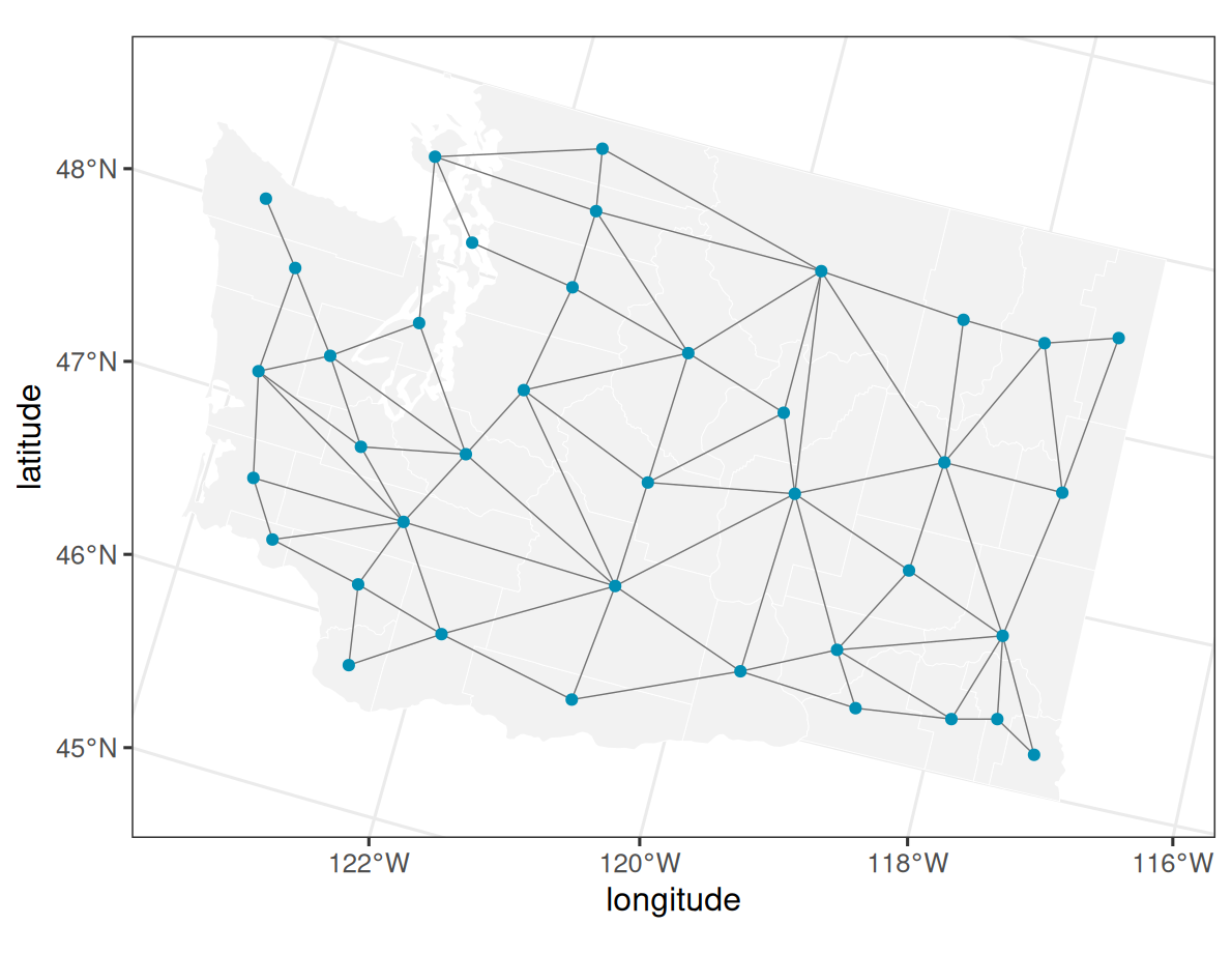

4 Negative-binomial data

We create a county covariate from east-west position, define a known exposure multiplier, and simulate a smooth areal effect from the proper CAR precision. Counts are generated from the negative-binomial model with fixed size \(r=12\). Four counties are held out by setting their observed response to NA; the rows stay in the data so their areal effects can be recovered and predicted.

Code

centroid_x <- sf::st_coordinates(sf::st_centroid(sf::st_geometry(wa_counties)))[, "X"]

dat_nb <- data.frame(
  area = as.character(wa_counties$COUNTYFIPS),
  county = wa_counties$COUNTYNM,
  x = as.numeric(scale(centroid_x))
)
dat_nb$log_exposure <- 0.25 * dat_nb$x

beta_nb <- c("(Intercept)" = 2.5, x = -0.35)
size_nb <- 12
sigma_sq_nb <- 1
rho_nb <- 0.9

Q_nb <- car_prec(g, sigma_sq = sigma_sq_nb, rho = rho_nb)
Sigma_nb <- solve(Q_nb)
w_nb <- rmvnorm(mean = rep(0, nrow(Q_nb)), Sigma = Sigma_nb)
names(w_nb) <- rownames(Q_nb)

dat_nb$w_true <- w_nb[dat_nb$area]
dat_nb$eta_true <- dat_nb$log_exposure +
  beta_nb["(Intercept)"] + beta_nb["x"] * dat_nb$x + dat_nb$w_true
dat_nb$mu_true <- exp(dat_nb$eta_true)
dat_nb$y_full <- rnbinom(nrow(dat_nb), size = size_nb, mu = dat_nb$mu_true)

holdout_nb <- sample(seq_len(nrow(dat_nb)), 4)
dat_nb$sample <- "training"
dat_nb$sample[holdout_nb] <- "holdout"
dat_nb$y <- dat_nb$y_full
dat_nb$y[holdout_nb] <- NA

Show plotting code

wa_nb <- wa_counties
wa_nb$area <- as.character(wa_nb$COUNTYFIPS)
wa_nb$y_full <- dat_nb$y_full[match(wa_nb$area, dat_nb$area)]
wa_nb$sample <- dat_nb$sample[match(wa_nb$area, dat_nb$area)]

ggplot(wa_nb) +
  geom_sf(aes(fill = y_full), color = "white", linewidth = 0.15) +
  geom_sf(
    data = wa_nb[wa_nb$sample == "holdout", ],
    fill = NA,
    color = "black",
    linewidth = 0.8
  ) +
  scale_fill_gradientn(colors = stlmm_palette()) +
  labs(fill = "count")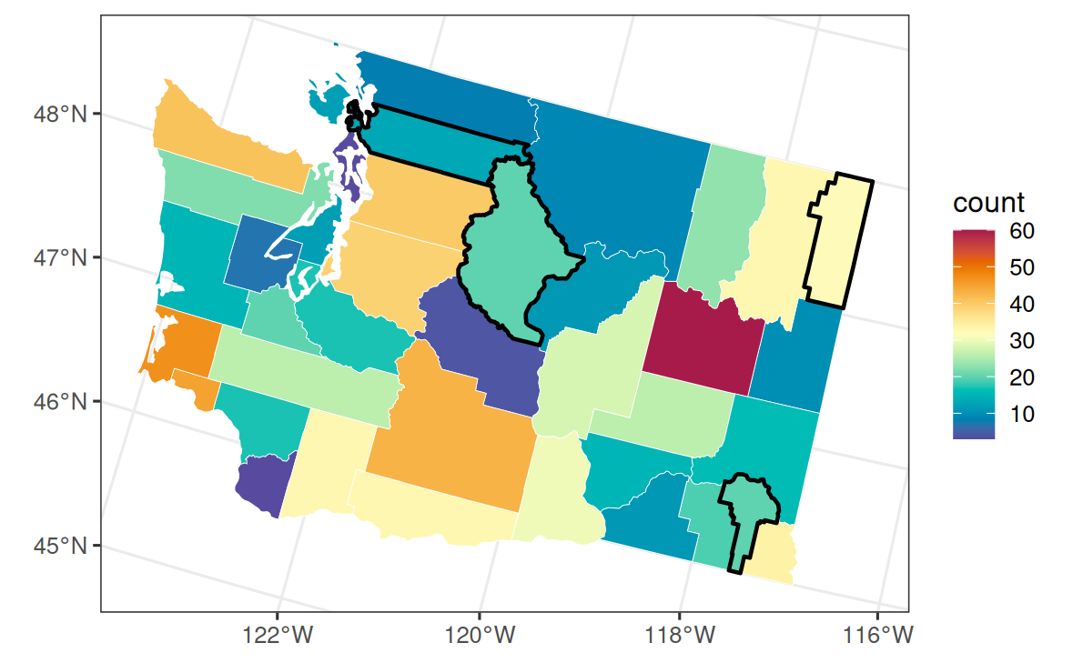

5 Fit the NB model

The family = "negative_binomial" argument selects the count likelihood, and size = size_nb fixes the negative-binomial size. There is no Gaussian residual variance term. The observation-level variability is defined by the count likelihood and the fixed size.

Code

fit_nb <- stLMM(
  y ~ x + offset(log_exposure) + car(area, graph = g),
  data = dat_nb,
  family = "negative_binomial",
  size = size_nb,
  priors = list(
    beta = normal(mean = 0, sd = 3),
    car_1 = list(
      sigma_sq = half_t(df = 3, scale = 1),
      rho = uniform(0.05, 0.95)
    )
  ),
  starting = list(car_1 = list(sigma_sq = 1, rho = 0.8)),
  tuning = list(car_1 = list(sigma_sq = 0.08, rho = 0.06)),
  n_samples = 1500,
  chains = 3,
  chain_control = list(seed = 14, dispersion = 1.5),
  verbose = FALSE
)

summary(fit_nb)

stLMM multi-chain summary
  formula: y ~ x + offset(log_exposure) + car(area, graph = g)
  chains: 3
  family: negative_binomial
  observations: 39 (35 observed, 4 missing response)
  posterior draws per chain: 1500
  process terms: 1

Parameters:
                  mean     sd    q2.5   q50.0  q97.5
(Intercept)     3.0064 0.1823  2.6290  3.0110 3.3543
x              -0.2199 0.1686 -0.5508 -0.2201 0.1135
car_1_sigma_sq  1.4354 0.5421  0.6105  1.3483 2.6561
car_1_rho       0.5108 0.2497  0.0751  0.5328 0.9167

Chain diagnostics:
                    parameter   rhat effective_size
(Intercept)       (Intercept) 1.0026      3562.4414
x                           x 1.0006      4232.1860
car_1_sigma_sq car_1_sigma_sq 1.0057       570.1364
car_1_rho           car_1_rho 1.0129       467.8318

Show trace-plot code

plot(
  fit_nb,
  parameters = trace_parameters,
  n_col = 2,
  burnin = 500,
  chain_colors = chain_colors
)

6 Recover areal effects

As with Gaussian CAR models, the structured CAR effect is integrated out during parameter updates. For Pólya-Gamma process models, stLMM() saves the in-chain process draws by default as save_process = list(start = 1, thin = 1) because those draws are already needed to refresh the augmentation variables. Calling recover() selects the retained county-effect draws requested by sub_sample; it does not run a separate post-fit Pólya-Gamma reconstruction. Use save_process = list(start = ..., thin = ...) to reduce memory use for larger process supports.

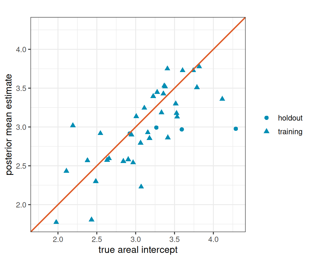
The intercept and the average level of a realized spatial effect can trade off, so the diagnostic below compares the areal intercept \(\beta_0 + w_i\) rather than \(w_i\) alone. The full log mean \(\eta_i = \beta_0 + x_i\beta_1 + w_i\) is often the more stable prediction-scale diagnostic, but \(\beta_0 + w_i\) is useful for seeing whether the structured surface is being recovered.

Code

rec_nb <- recover(fit_nb, sub_sample = list(start = 501, thin = 5))
rec_nb_draws <- as_samples(rec_nb, include_w = TRUE, metadata = FALSE)

w_nb_cols <- paste0("w_car_1_", seq_along(g$ids))
w_nb_hat <- colMeans(rec_nb_draws[, w_nb_cols, drop = FALSE])
names(w_nb_hat) <- g$ids
beta_nb_hat <- mean(rec_nb_draws[["(Intercept)"]])

nb_recovery <- data.frame(
  truth = beta_nb["(Intercept)"] + dat_nb$w_true,
  estimate = beta_nb_hat + w_nb_hat[dat_nb$area],
  sample = dat_nb$sample
)
head(nb_recovery)

         truth estimate   sample
53045 2.108637 2.432251 training
53053 3.155891 2.928566 training
53033 3.788620 3.509790 training
53005 3.515627 3.300382 training
53037 3.070838 2.228483 training
53007 3.593688 2.968485  holdout

Show plotting code

nb_recovery_lim <- range(nb_recovery$truth, nb_recovery$estimate)

ggplot(nb_recovery, aes(truth, estimate)) +
  geom_point(
    aes(shape = sample),
    color = stlmm_color("primary"),
    size = 2.2
  ) +
  geom_abline(
    intercept = 0,
    slope = 1,
    color = stlmm_color("secondary"),
    linewidth = 0.8
  ) +
  coord_equal(xlim = nb_recovery_lim, ylim = nb_recovery_lim) +
  labs(
    x = "true areal intercept",
    y = "posterior mean estimate",
    shape = NULL
  )

7 Fitted means and holdout counts

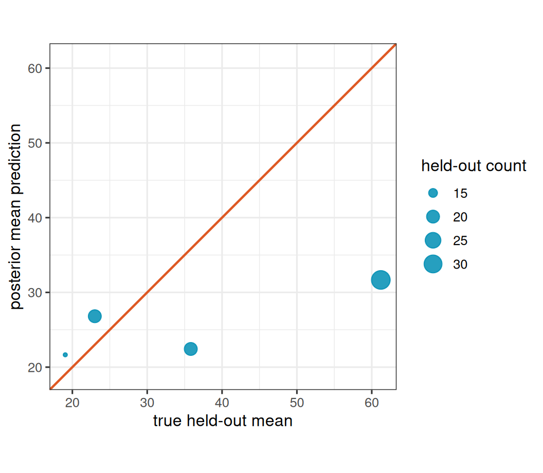
The default response scale for negative-binomial models is the mean count \(\mu_i = \exp(\eta_i)\). The link scale is the log mean.

Code

fitted_nb <- fitted(rec_nb)
fitted_nb_link <- fitted(rec_nb, scale = "link")

head(data.frame(mean_count = fitted_nb, log_mean = fitted_nb_link))

  mean_count log_mean
1   11.68678 2.395298
2   19.12890 2.905980
3   34.13492 3.494687
4   28.44876 3.313113
5   10.04859 2.228343
6   22.43207 2.973612

Code

holdout_nb_new <- dat_nb[holdout_nb, c("area", "x", "log_exposure")]

pred_nb <- predict(
  rec_nb,
  newdata = holdout_nb_new,
  y_samples = TRUE
)

summary(pred_nb)

stLMM multi-chain prediction summary
  chains: 3
  pooled draws: 600
  rows: 4
  newdata: TRUE

mu:
      mean      sd   q2.5   q50.0    q97.5
37 26.8111 21.3066 5.5114 20.7274  80.5173
6  22.4321 13.4192 6.3866 19.2199  53.5082
9  21.6516 13.6835 5.7979 18.2006  56.4631
17 31.6663 43.2377 3.2730 21.1770 126.3192

y:
      mean      sd q2.5 q50.0   q97.5
37 27.3667 25.6338    4    20  93.000
6  22.1683 16.2809    4    18  59.050
9  21.8783 16.1521    4    18  64.000
17 31.5300 48.6842    2    20 127.075

Show plotting code

pred_nb_mu <- as_samples(pred_nb, sample = "mu", metadata = FALSE)
pred_nb_dat <- data.frame(
  mu = dat_nb$mu_true[holdout_nb],
  mu_hat = colMeans(pred_nb_mu),
  y = dat_nb$y_full[holdout_nb]
)
pred_nb_lim <- range(pred_nb_dat$mu, pred_nb_dat$mu_hat)

ggplot(pred_nb_dat, aes(mu, mu_hat)) +
  geom_point(aes(size = y), color = stlmm_color("primary"), alpha = 0.85) +
  geom_abline(
    intercept = 0,
    slope = 1,
    color = stlmm_color("secondary"),
    linewidth = 0.8
  ) +
  coord_equal(xlim = pred_nb_lim, ylim = pred_nb_lim) +
  labs(
    x = "true held-out mean",
    y = "posterior mean prediction",
    size = "held-out count"
  )

8 Poisson data and a large-size approximation

If \(r\) is large, the negative-binomial variance \(\mu_i + \mu_i^2/r\) is close to the Poisson variance \(\mu_i\). This section simulates Poisson counts on the same county support and fits a negative-binomial model with a large fixed size. This is useful as a diagnostic for the approximation, not a replacement for a dedicated Poisson likelihood.

Code

set.seed(1)

dat_pois <- dat_nb[, c("area", "county", "x", "log_exposure")]

beta_pois <- c("(Intercept)" = 5, x = -0.5)
sigma_sq_pois <- 1
rho_pois <- 0.9
size_pois_approx <- 1000

Q_pois <- car_prec(g, sigma_sq = sigma_sq_pois, rho = rho_pois)
Sigma_pois <- solve(Q_pois)
w_pois <- rmvnorm(mean = rep(0, nrow(Q_pois)), Sigma = Sigma_pois)
names(w_pois) <- rownames(Q_pois)

dat_pois$w_true <- w_pois[dat_pois$area]
dat_pois$eta_true <- dat_pois$log_exposure +
  beta_pois["(Intercept)"] + beta_pois["x"] * dat_pois$x + dat_pois$w_true
dat_pois$mu_true <- exp(dat_pois$eta_true)
dat_pois$y <- rpois(nrow(dat_pois), lambda = dat_pois$mu_true)

Show plotting code

wa_pois <- wa_counties
wa_pois$area <- as.character(wa_pois$COUNTYFIPS)
wa_pois$y <- dat_pois$y[match(wa_pois$area, dat_pois$area)]

ggplot(wa_pois) +
  geom_sf(aes(fill = y), color = "white", linewidth = 0.15) +
  scale_fill_gradientn(colors = stlmm_palette()) +
  labs(fill = "count")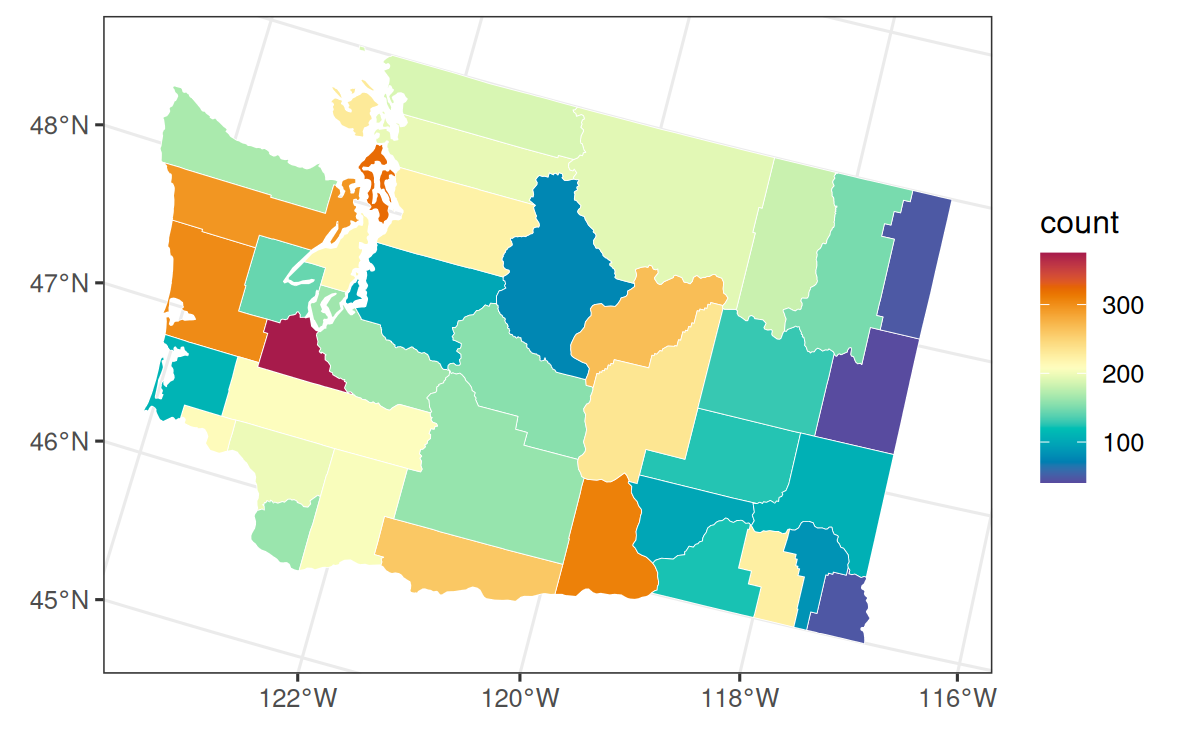

Code

fit_pois_nb <- stLMM(
  y ~ x + offset(log_exposure) + car(area, graph = g),
  data = dat_pois,
  family = "negative_binomial",
  size = size_pois_approx,
  priors = list(
    beta = normal(mean = 0, sd = 3),
    car_1 = list(
      sigma_sq = half_t(df = 3, scale = 1),
      rho = uniform(0.05, 0.95)
    )
  ),
  starting = list(car_1 = list(sigma_sq = 1, rho = 0.8)),
  tuning = list(car_1 = list(sigma_sq = 0.08, rho = 0.06)),
  n_samples = 1200,
  chains = 3,
  chain_control = list(seed = 15, dispersion = 1.5),
  verbose = FALSE
)

summary(fit_pois_nb)

stLMM multi-chain summary
  formula: y ~ x + offset(log_exposure) + car(area, graph = g)
  chains: 3
  family: negative_binomial
  observations: 39
  posterior draws per chain: 1200
  process terms: 1

Parameters:
                  mean     sd    q2.5   q50.0   q97.5
(Intercept)     5.0982 0.1151  4.8612  5.0999  5.3252
x              -0.4967 0.1123 -0.7185 -0.4984 -0.2680
car_1_sigma_sq  0.7476 0.1927  0.4467  0.7228  1.1973
car_1_rho       0.5109 0.2279  0.0913  0.5125  0.9081

Chain diagnostics:
                    parameter   rhat effective_size
(Intercept)       (Intercept) 1.0011      3773.6980
x                           x 1.0000      3576.7674
car_1_sigma_sq car_1_sigma_sq 1.0183       413.6985
car_1_rho           car_1_rho 1.0028       323.2603

Show trace-plot code

plot(
  fit_pois_nb,
  parameters = trace_parameters,
  n_col = 2,
  burnin = 400,
  chain_colors = chain_colors
)

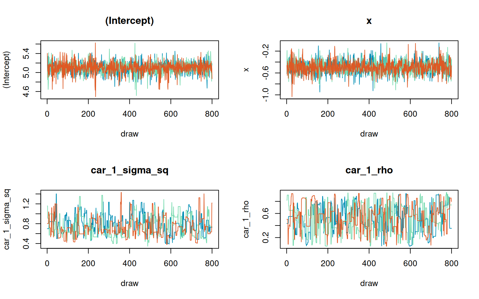
Code

rec_pois_nb <- recover(fit_pois_nb, sub_sample = list(start = 401, thin = 4))
rec_pois_draws <- as_samples(rec_pois_nb, include_w = TRUE, metadata = FALSE)

w_pois_hat <- colMeans(rec_pois_draws[, w_nb_cols, drop = FALSE])
names(w_pois_hat) <- g$ids
beta_pois_hat <- mean(rec_pois_draws[["(Intercept)"]])

pois_recovery <- data.frame(
  truth = beta_pois["(Intercept)"] + dat_pois$w_true,
  estimate = beta_pois_hat + w_pois_hat[dat_pois$area]
)

Show plotting code

pois_recovery_lim <- range(pois_recovery$truth, pois_recovery$estimate)

ggplot(pois_recovery, aes(truth, estimate)) +
  geom_point(color = stlmm_color("primary"), size = 2.2) +
  geom_abline(
    intercept = 0,
    slope = 1,
    color = stlmm_color("secondary"),
    linewidth = 0.8
  ) +
  coord_equal(xlim = pois_recovery_lim, ylim = pois_recovery_lim) +
  labs(
    x = "true areal intercept",
    y = "posterior mean estimate"
  )

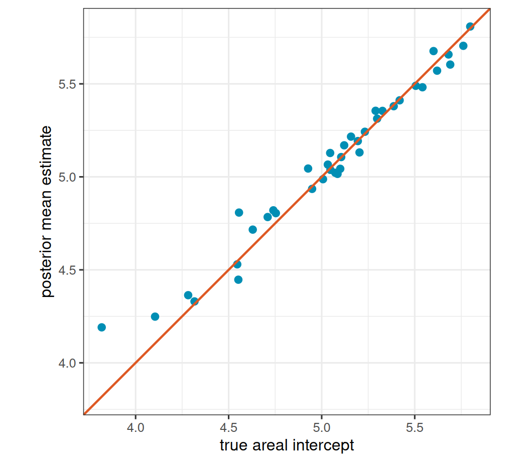
The large-size fit uses the same package machinery as the negative-binomial example. In this small simulation it should recover the log mean surface reasonably well, but the approximation is still an NB model. In applications where a Poisson likelihood is the scientific target, a native Poisson implementation would be the cleaner model.

9 Practical guidance

The fixed-size negative-binomial family is useful when counts are overdispersed relative to Poisson and a fixed size is scientifically defensible or can be sensitivity-tested. A simple workflow is to fit a small grid of plausible sizes and compare fixed effects, fitted means, spatial variance, and recovered areal intercepts.

The size parameter also interacts with random and structured effects. Smaller size gives extra observation-level overdispersion, while spatial random effects explain persistent area-level variation. Because these components can trade off, report sensitivity to size when the data do not strongly determine the distinction.

Very large size values approximate Poisson counts, but they are not automatically better. The Pólya-Gamma draw has shape \(y_i + r\), so large size can increase computational cost or change sampler behavior. Use a large-size NB fit as an approximation check, not as a blanket recommendation.

For negative-binomial models, fitted() and predict() return mean counts on the response scale by default. Use scale = "link" for the log mean. If y_samples = TRUE, prediction simulates negative-binomial count outcomes using the fixed size.

Polson, Nicholas G., James G. Scott, and Jesse Windle. 2013. “Bayesian Inference for Logistic Models Using Pólya-Gamma Latent Variables.” Journal of the American Statistical Association 108 (504): 1339–49. https://doi.org/10.1080/01621459.2013.829001.

Windle, Jesse, Carlos M. Carvalho, James G. Scott, and Liyun Sun. 2013. “Efficient Data Augmentation in Dynamic Models for Binary and Count Data.” arXiv Preprint arXiv:1308.0774. https://arxiv.org/abs/1308.0774.