
Metropolis blocking and adaptation in stLMM
How covariance and residual-variance proposals are tuned, blocked, and diagnosed
Source:vignettes/a10-metropolis-blocking-diagnostics.qmd
1 Overview
This vignette focuses on the Metropolis part of the stLMM sampler: which parameters enter it, how proposals are adapted, what the blocking options do, and how to decide whether a blocking scheme is worth the added computing time.
The discussion is about the sampler implemented in stLMM, not a claim that the collapsed parameterization is best for every model or even the most natural parameterization for blocking. Similar models, and much more sophisticated hierarchical models, can be fit in general Bayesian modeling software. Those tools can represent the model in different ways: latent variables may be retained as parameters, centered or non-centered parameterizations may be used, and groups of model nodes or parameters may be updated with customized samplers. Those choices can be more favorable for a particular posterior geometry (Papaspiliopoulos et al. 2007; Stan Development Team 2025). Software built around programmable model graphs, such as NIMBLE, exposes this kind of sampler customization and even automated blocking because useful blocks are model- and parameterization-specific (Valpine et al. 2017; NIMBLE Development Team 2026).
The useful role for stLMM is narrower. It gives formula-level access to a specific family of spatial and space-time linear mixed models, including structured covariance terms, NNGP approximations, residual-variance options used in small area estimation, recovery and prediction methods, and fixed-parameter controls. The aim is to make these models easier to fit without requiring users to write the full latent model and sampler themselves. The collapsed sampler reduces the Markov chain dimension and gives one coherent implementation across these terms, but blocking then operates only on the covariance and residual-variance parameters through the collapsed target. That can be an advantage for routine models and a limitation for difficult posterior geometries.
stLMM uses a collapsed sampler for structured latent process terms such as ar1(), gp(), nngp(), car(), and car_time(). The uncollapsed Gaussian model can be written as
\[ \mathbf{y} = \mathbf{X}\mathbf{\beta} + \mathbf{Z}\mathbf{\alpha} + \mathbf{A}\mathbf{w} + \mathbf{\varepsilon}, \]
\[ \mathbf{w} \sim N(\mathbf{0}, \mathbf{Q}_w^{-1}), \qquad \mathbf{\varepsilon} \sim N(\mathbf{0}, \mathbf{R}), \]
where \(\mathbf{A}\) maps observation rows to structured latent process nodes, \(\mathbf{Q}_w\) is the structured-process prior precision, \(\mathbf{R}\) is the diagonal residual covariance, and \(\mathbf{W}=\mathbf{R}^{-1}\) is the diagonal observation precision. Under the default homoskedastic Gaussian residual model, \(\mathbf{R}=\tau^2\mathbf{I}_n\) and \(\mathbf{W}=\tau^{-2}\mathbf{I}_n\).
During fitting, the structured process vector \(\mathbf{w}\) isn’t sampled while covariance parameters are updated. Instead, \(\mathbf{w}\) is integrated out. We reserve \(\mathbf{\theta}_k\) for the covariance-function parameters of structured process term \(k\), such as a range, decay, correlation, smoothness, or nonseparable mixing parameter. The broader Metropolis-updated parameter collection is denoted \(\mathbf{\psi}\); it can include \(\tau^2\), residual variances, process variances \(\sigma_k^2\), and \(\mathbf{\theta}_k\) values. Conditional on \(\mathbf{\beta}\), \(\mathbf{\alpha}\), and \(\mathbf{\psi}\), the collapsed observation model is
\[ \mathbf{y} \mid \mathbf{\beta}, \mathbf{\alpha}, \mathbf{\psi} \sim N(\mathbf{X}\mathbf{\beta} + \mathbf{Z}\mathbf{\alpha}, \mathbf{V}), \]
with
\[ \mathbf{V} = \mathbf{R} + \mathbf{A}\mathbf{Q}_w^{-1}\mathbf{A}^{\top}. \]
The code doesn’t form \(\mathbf{V}\) explicitly; rather, it evaluates the collapsed target through the sparse latent matrix
\[ \mathbf{M} = \mathbf{Q}_w + \mathbf{A}^{\top}\mathbf{W}\mathbf{A}, \]
which gives
\[ \begin{aligned} \mathbf{V}^{-1} &= \mathbf{W} - \mathbf{W}\mathbf{A}\mathbf{M}^{-1} \mathbf{A}^{\top}\mathbf{W}, \\ \log|\mathbf{V}| &= \log|\mathbf{R}| + \log|\mathbf{M}| - \log|\mathbf{Q}_w|. \end{aligned} \]
The dependence of \(\mathbf{R}\), \(\mathbf{W}\), \(\mathbf{Q}_w\), \(\mathbf{V}\), and \(\mathbf{M}\) on the current value of \(\mathbf{\psi}\) is suppressed to keep the notation readable.
This collapsed-sampler choice is deliberate, but it has real costs. It reduces the retained MCMC parameter space and lets stLMM fit several structured random-effect models in one framework, including dense GP, NNGP, AR(1), CAR, CAR-time, and covariate-scaled process terms. Once \(\mathbf{w}\) is integrated out, however, many covariance and variance parameters don’t have simple Gibbs updates. A proposed range, correlation, mixing, process-variance, or residual-variance value has to be evaluated through the collapsed target, which can require rebuilding covariance or precision pieces, assembling \(\mathbf{M}\), and factorizing \(\mathbf{M}\).
Blocking is the choice of which Metropolis-updated parameters are proposed together. One large block can be efficient when posterior dependence is well captured by the adaptive proposal covariance, but it can struggle when different parameter groups move on different scales or have different posterior dependence patterns. Splitting parameters into smaller blocks can sometimes improve mixing because each proposal is tuned to a more focused part of the posterior. There is no free lunch: each extra Metropolis block can add another target evaluation and factorization within the same retained iteration.
After collapsing the structured process terms, only a few parameter groups have Gibbs updates:
- fixed effects \(\mathbf{\beta}\) are updated by Gibbs steps;
- unstructured grouped random effects \(\mathbf{\alpha}\), when included through terms such as
iid(group), are updated by Gibbs steps; - structured process effects \(\mathbf{w}\) are recovered after fitting with
recover(), not sampled during covariance-parameter updates.
The default Metropolis update is one joint block containing the covariance and residual-variance parameters that are updated by Metropolis. That’s usually fastest. Splitting the parameters into several blocks can improve mixing when one large proposal is hard to tune, but it can make each iteration more expensive. Blocking is therefore a computational tradeoff, not a universally better sampler.
The retained adaptive Metropolis strategy used in stLMM adapts ideas from unpublished adaptive Metropolis notes by Benjamin Shaby and from the broader adaptive MCMC literature (Andrieu and Thoms 2008).
stLMM records sampler timing in the returned fit object. For a single-chain fit, fit$timing$sampler gives the usual proc.time() CPU and elapsed wall-clock differences around the compiled sampler call. For a multi-chain fit, fit$timing$sampler_by_chain gives those values by chain and fit$timing$sampler_total gives the total across chains. We’ll use those values below to compare the computational cost of blocking schemes.
2 What Enters the Metropolis Update
The Metropolis machinery only sees covariance and residual-variance parameters that are updated during MCMC. Fixed parameters declared with fixed(value) are omitted from every Metropolis block. They stay at their fixed values and don’t need priors.
The sampler proposes on transformed scales. Positive parameters, such as \(\tau^2\) and process variances, are updated on the log scale. Bounded covariance-function parameters are updated on a bounded-logit scale. For example, in an exponential NNGP model with residual variance, process variance, and spatial decay all updated by Metropolis, one possible transformed vector is
\[ \mathbf{\eta} = \{\log(\tau^2), \log(\sigma^2), g(\phi)\}^{\top}, \]
where \(\phi\) is the term’s decay parameter and \(g(\cdot)\) maps its bounded prior support to the real line. In general, \(\mathbf{\eta}\) contains the transformed parameters that are updated by Metropolis. Priors and transformation Jacobians are included in the Metropolis target, so proposals are made on convenient scales while the posterior remains the model specified by the user.
3 The Adaptive Metropolis Step
Let \(\mathbf{\eta}_b\) be the current transformed parameter vector for block \(b\). All parameters outside block \(b\) are held fixed while that block is proposed. Let \(\ell(\mathbf{\eta}_b)\) denote the collapsed log posterior target under the current block values, including the collapsed likelihood, priors, and transformation Jacobians.
For each retained MCMC iteration, the sampler loops over the Metropolis blocks. For each block \(b\):
- Propose a random walk on the transformed scale,
\[ \mathbf{\eta}_b^\star = \mathbf{\eta}_b + \mathbf{L}_b \mathbf{z}, \qquad \mathbf{z} \sim N(\mathbf{0}, \mathbf{I}). \]
For multivariate blocks, \(\mathbf{L}_b\mathbf{L}_b^{\top}=\lambda_b\mathbf{\Sigma}_b\), where \(\mathbf{\Sigma}_b\) is the adaptive empirical covariance shape and \(\lambda_b\) is a variance-like multiplier. For scalar blocks, the proposal variance is \(\delta_b^2\Sigma_b\), where \(\Sigma_b>0\) is a scalar shape and \(\delta_b\) is a one-dimensional random-walk scale. The two symbols reflect the implementation: multivariate blocks adapt an empirical covariance shape and a multiplier on that covariance, while scalar blocks adapt a direct step size.
Transform \(\mathbf{\eta}_b^\star\) back to the model scale.
Rebuild the affected covariance or precision pieces, assemble \(\mathbf{M}\), and factorize it. If the proposed covariance or precision isn’t valid, reject the proposal.
Otherwise accept with probability
\[ \min\left\{ 1, \exp\left[ \ell(\mathbf{\eta}_b^\star) - \ell(\mathbf{\eta}_b) \right] \right\}. \]
- At the end of each retained adaptation batch, compute the block acceptance rate \(\hat{a}_b\). For multivariate blocks, update the proposal multiplier and empirical covariance by
\[ \log(\lambda_b) \leftarrow \log(\lambda_b) + c_0 (m+1)^{-c_1}(\hat{a}_b-a^\star), \]
\[ \mathbf{\Sigma}_b \leftarrow \mathbf{\Sigma}_b + (m+1)^{-c_1} (\widehat{\mathrm{Cov}}_b-\mathbf{\Sigma}_b), \]
where \(m\) is the completed batch index, \(a^\star\) is the target acceptance rate, and the implementation uses \(c_0=1\) and \(c_1=0.8\).
Scalar blocking uses one-dimensional scale adaptation for \(\delta_b\) and defaults to target acceptance 0.44. Multivariate blocking defaults to target acceptance 0.234. The adaptation is diminishing, so later batches make smaller changes. Diminishing adaptation is one of the standard conditions used in adaptive MCMC theory; paired with suitable control of the proposal kernels, it helps preserve ergodicity while allowing the proposal to keep learning during the run (Roberts and Rosenthal 2007, 2009).
4 Warmup and Retained Adaptation
There are two tuning phases, and they serve different purposes.
First, the warmup phase adjusts proposal scales before retained samples are collected. Warmup draws aren’t returned as posterior samples, but warmup diagnostics are stored in fit$adaptive_metropolis$warmup. In the next phase, retained adaptation continues during the posterior run. Its diagnostics are stored in fit$adaptive_metropolis and, for blocked updates, in fit$adaptive_metropolis$blocks. See ?stLMM for the full set of warmup and metropolis controls and their defaults.
5 Blocking Choices
Blocking changes the proposal partition. It doesn’t change the model, likelihood, prior, or posterior target.
| Blocking | Partition | Use |
|---|---|---|
| "joint" | All covariance and residual-variance parameters updated by Metropolis in one block. | Start here; usually fastest. |
| "by_term" | Residual variance in one block; each structured process term's variance and covariance-function parameters in its own block. | Several process terms appear to tune differently. |
| "residual_process" | Residual variances in one block; process covariance parameters in another. | Residual variances dominate the joint proposal. |
| "variance_theta" | Variance parameters, including residual and process variances, in one block; bounded covariance parameters in another. | Variance-like parameters and bounded covariance-function parameters move differently. |
| "process_variance" | Residual variance in one block; process variances in one block; bounded covariance parameters in one block. | Residual variance, process variance, and covariance-function parameters each need separate movement. |
| "scalar" | Each covariance or residual-variance parameter is updated individually in its own one-dimensional block. | Diagnostic fallback when larger blocks don't move. |
5.1 A Diagnostic NNGP Example
The example below uses one spatial NNGP term. The Metropolis-updated parameters are the residual variance tau_sq, the process variance nngp_1_sigma_sq, and the spatial decay nngp_1_phi.
This is a useful diagnostic example because the two variance parameters can move differently from the decay parameter. We’ll compare:
-
"joint", the default, which updates all three parameters together; -
"by_term", which updatestau_sqby itself, then updatesnngp_1_sigma_sqandnngp_1_phitogether.
Code
n <- 200

dat <- data.frame(
  x_coord = runif(n),
  y_coord = runif(n),
  x = runif(n, -1, 1)
)

beta <- c(0.5, 1)
tau_sq <- 0.1
sigma_sq <- 0.5
phi <- 5

C <- exp_cov(
  dat[, c("x_coord", "y_coord")],
  sigma_sq = sigma_sq,
  phi = phi
)

w <- rmvnorm(mean = rep(0, n), Sigma = C)
mu <- beta[1] + beta[2] * dat$x + w
dat$y <- mu + rnorm(n, sd = sqrt(tau_sq))
The chains are short enough for a vignette, but long enough to show the blocking tradeoff without relying on a specially selected data realization. We set chain_control$dispersion above its default to start the chains farther apart for the positive variance parameters. In a real analysis, use longer chains and don’t make a blocking decision from one run alone.
Code
fit_with_blocking <- function(blocking){
  stLMM(
    y ~ x + nngp(x_coord, y_coord, m = 15,
                 cov_model = "exp", ordering = "maxmin"),
    data = dat,
    priors = list(
      resid = list(tau_sq = half_t(df = 3, scale = 0.5)),
      nngp_1 = list(
        sigma_sq = half_t(df = 3, scale = 1),
        phi = uniform(1, 15)
      )
    ),
    n_samples = 1500,
    chains = 3,
    chain_control = list(seed = 1, dispersion = 2),
    metropolis = list(
      blocking = blocking,
      batch_length = 25
    ),
    verbose = FALSE
  )
}
Code
joint_run <- fit_with_blocking("joint")
by_term_run <- fit_with_blocking("by_term")
5.2 Compare Blocking Diagnostics
First check the blocks used by the first chain. The table reports the model-scale parameter names so the grouping is easy to read.
| Blocking | Block | Dimension | Acceptance | Parameters |
|---|---|---|---|---|
| joint | 1 | 3 | 0.264 | tau_sq, nngp_1_sigma_sq, nngp_1_phi |
| by_term | 1 | 1 | 0.323 | tau_sq |
| by_term | 2 | 2 | 0.244 | nngp_1_sigma_sq, nngp_1_phi |
Next use multi-chain diagnostics. summary() for a multi-chain stLMM fit reports diagnostics computed with coda, and as_mcmc() returns a coda::mcmc.list if you want to work directly with the chains. The burn and thin arguments can be passed to as_mcmc() directly, including for recovered multi-chain objects. Here we focus on \(\hat R\), effective sample size (ESS), and ESS per second for the Metropolis-updated parameters.
| Blocking | Parameter | Rhat | ESS | ESS per second |
|---|---|---|---|---|
| joint | tau_sq | 1.028 | 362.8 | 65.8 |
| joint | nngp_1_sigma_sq | 1.097 | 240.3 | 43.6 |
| joint | nngp_1_phi | 1.028 | 248.2 | 45.0 |
| by_term | tau_sq | 1.015 | 347.5 | 31.5 |
| by_term | nngp_1_sigma_sq | 1.078 | 361.8 | 32.8 |
| by_term | nngp_1_phi | 1.016 | 289.4 | 26.3 |
It’s also helpful to summarize the cost of each blocking scheme. A blocked sampler can have better convergence diagnostics per retained iteration but still lose on effective sample size per second if the extra blocks make each iteration much slower.
| Blocking | Sampler elapsed seconds | Worst Rhat | Minimum ESS | Minimum ESS per second |
|---|---|---|---|---|
| joint | 5.51 | 1.097 | 240.3 | 43.6 |
| by_term | 11.01 | 1.078 | 289.4 | 26.3 |
In this example, the default joint block is the baseline: it keeps the process variance and decay parameter in the same proposal and avoids extra target evaluations. The "by_term" option asks a specific question: does the residual variance need to move separately from the NNGP covariance parameters? In this run, the answer is no. The added block costs more computation and doesn’t improve the chain diagnostics enough to beat the default joint update. That is the teaching point. Blocking can be useful, but it has to earn its cost in better mixing, higher ESS, or better ESS per second.
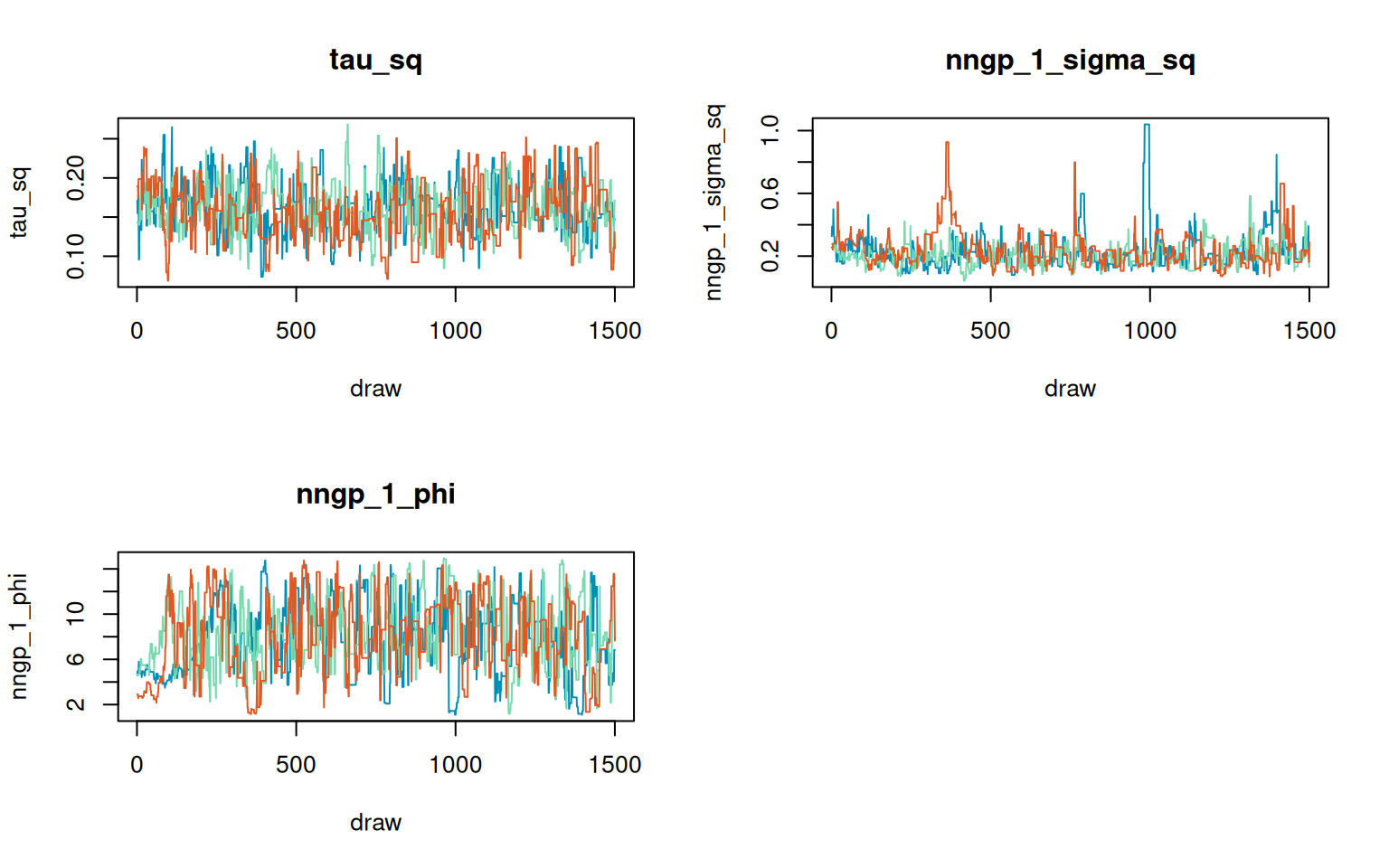
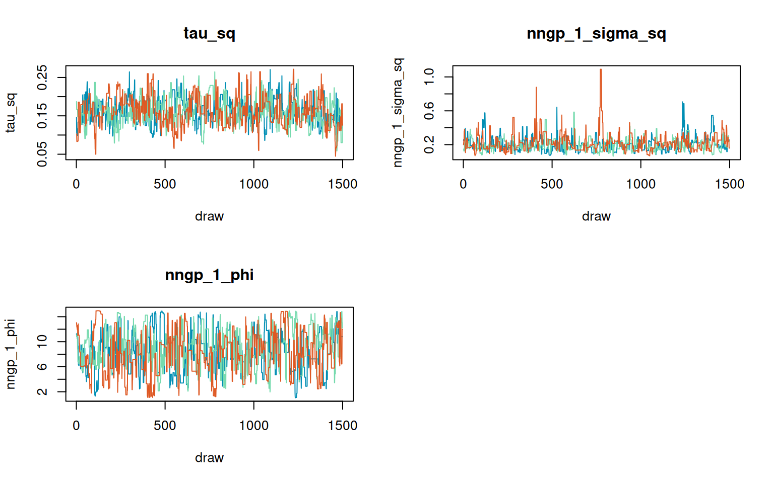
Trace plots are still worth looking at. \(\hat R\) and ESS can miss local behavior, especially in short runs.
Show joint run plotting code
chain_colors <- stlmm_discrete_colors(3)

plot(
  joint_run,
  parameters = covariance_parameters,
  n_col = 2,
  chain_colors = chain_colors
)
Show by_term run plotting code
plot(
  by_term_run,
  parameters = covariance_parameters,
  n_col = 2,
  chain_colors = chain_colors
)
6 Changing Adaptation Settings
The previous fits used the default retained target acceptance for multivariate blocks. You can change retained adaptation through the metropolis list. The call below uses "variance_theta" blocking, longer retained adaptation batches, and a slightly higher target acceptance rate.
Code
fit_custom <- stLMM(
  y ~ x + nngp(x_coord, y_coord, m = 15,
               cov_model = "exp", ordering = "maxmin"),
  data = dat,
  priors = list(
    resid = list(tau_sq = half_t(df = 3, scale = 0.5)),
    nngp_1 = list(
      sigma_sq = half_t(df = 3, scale = 1),
      phi = uniform(1, 15)
    )
  ),
  warmup = list(
    batch_length = 50,
    min_batches = 3,
    max_batches = 30,
    target = c(0.20, 0.40)
  ),
  metropolis = list(
    blocking = "variance_theta",
    batch_length = 50,
    target_accept = 0.30
  )
)
The scalar option is available too.
Scalar updates can help diagnose whether a multivariate block is too hard to tune. They shouldn’t be treated as a routine default for collapsed process models because each scalar proposal can require another collapsed target evaluation and factorization of \(\mathbf{M}\).
7 Practical Guidance
Start with "joint". It’s the default because it’s usually fastest and often mixes well enough.
Try "variance_theta" when variance-like parameters and bounded range or correlation parameters appear to move on different scales. This is a common first alternative for a single structured process term.
Try "by_term" when a model has several structured process terms and one term appears to tune differently from the others.
Try "process_variance" when residual variance, process variance, and range or correlation parameters each need separate movement.
Try "residual_process" when residual variances dominate the joint proposal.
Use "scalar" as a diagnostic fallback. It can improve movement for stubborn parameters, but it can be much slower because it may multiply the number of collapsed target evaluations per retained iteration.
Compare blocking choices with several criteria: trace plots, block acceptance rates, \(\hat R\), effective sample size, effective sample size per second, posterior summaries, and runtime. Better mixing per iteration only helps if it improves mixing enough to justify the extra target evaluations.
For difficult models, treat blocking as one diagnostic tool among several rather than as evidence that one parameterization is uniformly better.