Purpose
This vignette compares the ICAR model used in the NIMBLE Scottish lip cancer case study with three stLMM count-model alternatives: large-size negative-binomial approximations with proper CAR, Leroux CAR, and DAGAR latent effects. The goal is to see how close the stLMM SIR estimates are to the NIMBLE ICAR estimates when the models target the same relative-risk surface but use related, nonidentical spatial priors.
The NIMBLE reference model is
\[
\begin{aligned}
O_i \mid \lambda_i &\sim \operatorname{Poisson}(\lambda_i E_i),\\
\log(\lambda_i) &= \alpha + \phi_i,\\
𝛟 &\sim \operatorname{ICAR}(\mathbf{W}, 1/\tau_\phi).
\end{aligned}
\]
The stLMM proper CAR model is
\[
\begin{aligned}
O_i &\sim \operatorname{NB}(\mu_i, r),\\
\log(\mu_i) &= \log(E_i) + \alpha + w_i,\\
\mathbf{w} &\sim N\{0, \sigma^2(\mathbf{D}-\rho\mathbf{G})^{-1}\}.
\end{aligned}
\]
The stLMM Leroux CAR model uses
\[
\begin{aligned}
O_i &\sim \operatorname{NB}(\mu_i, r),\\
\log(\mu_i) &= \log(E_i) + \alpha + w_i,\\
\mathbf{w} &\sim N\{0, \sigma^2[(1-\rho)\mathbf{I}+\rho(\mathbf{D}-\mathbf{G})]^{-1}\}.
\end{aligned}
\]
The stLMM DAGAR model uses the same likelihood and offset but replaces the CAR prior with a directed areal prior,
\[
\begin{aligned}
O_i &\sim \operatorname{NB}(\mu_i, r),\\
\log(\mu_i) &= \log(E_i) + \alpha + w_i,\\
\mathbf{w} &\sim N\{0, \sigma^2\mathbf{Q}_{\operatorname{DAGAR}}(\rho; \mathbf{G}, \mathcal{O})^{-1}\},
\end{aligned}
\]
where \(\mathcal{O}\) is the ordering used to orient the graph.
All fitted models estimate the same response-scale target,
\[
\lambda_i = \mu_i/E_i,
\]
the standardized incidence ratio (SIR). The main modeling differences to keep in mind are:
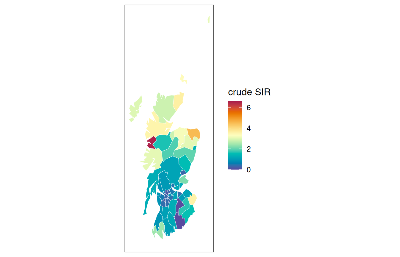
- crude SIR, \(O_i/E_i\), is very noisy where expected counts are small;
- NIMBLE uses an exact Poisson likelihood and an intrinsic, sum-constrained CAR prior;
- stLMM uses a large-size NB likelihood and proper CAR, Leroux CAR, or DAGAR priors;
- the GeoDa graph has disconnected components and isolated regions, while the stLMM fits use a connected graph with nearest-neighbor bridge edges.
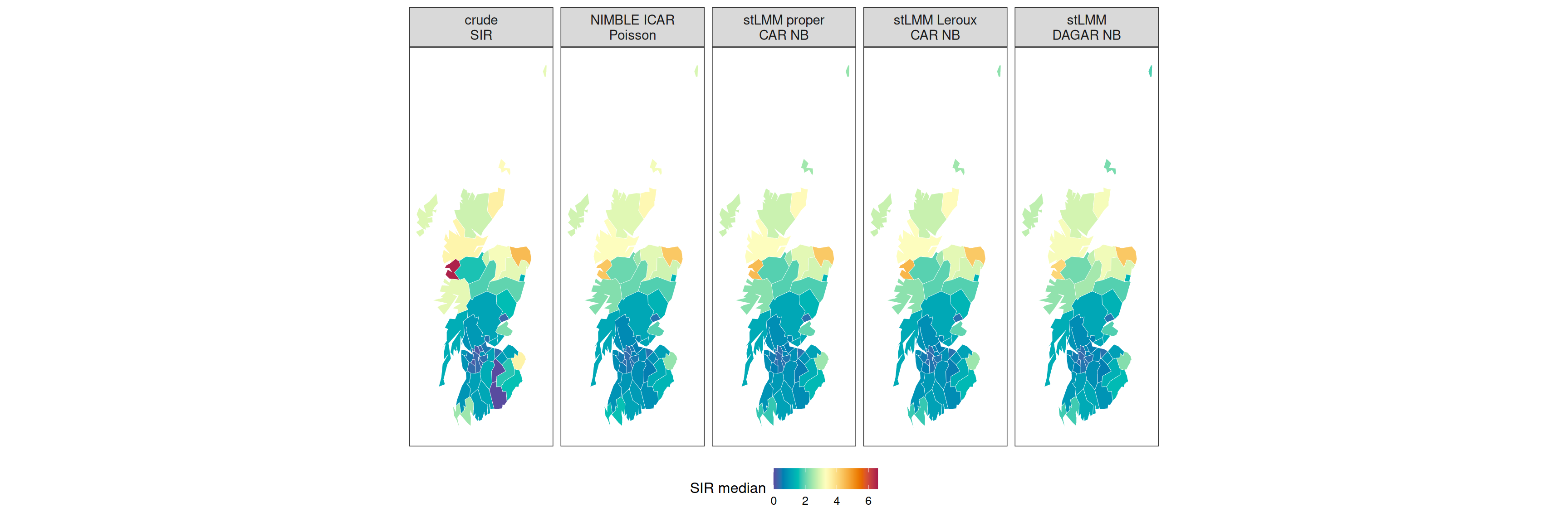
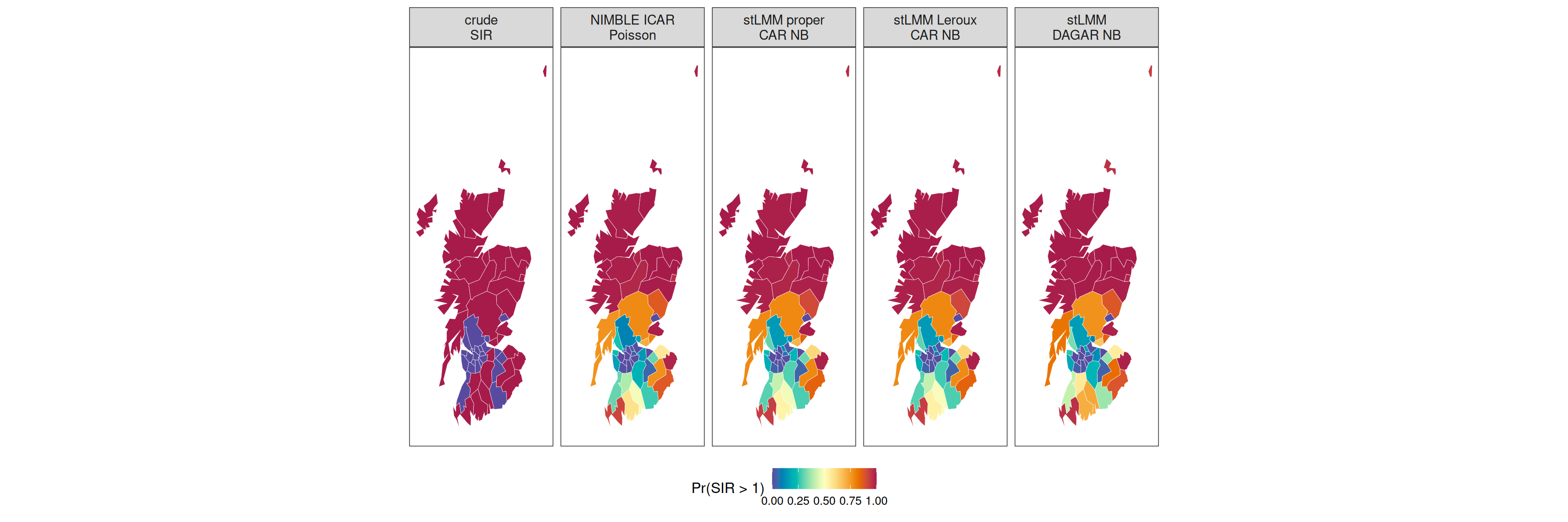
These differences are enough that the fitted SIR surfaces should be expected to show similar broad smoothing behavior, not identical estimates.
Requirements
The NIMBLE comparison requires nimble and the packages needed to compile and run NIMBLE models. Those packages are not stLMM requirements; they are needed only when params$run_nimble is true. Install nimble before rendering the full comparison:
The two samplers use different implementations, but the comparison below uses the same number of chains, the same total chain length, and the same number of retained posterior draws per chain for each fitted model. Each chain runs for 10,000 total iterations, with the first 5,000 discarded and every 25th remaining draw retained for summaries.
Code
data.frame(
  sampler = c("NIMBLE ICAR", "stLMM CAR/DAGAR"),
  chains = n_chains,
  discard = c(burnin_nimble, burnin_stlmm),
  thin = c(thin_nimble, thin_stlmm),
  iter_per_chain = c(niter_nimble, niter_stlmm),
  kept_per_chain = n_keep_per_chain,
  kept_total = n_chains * n_keep_per_chain
) |>
  knitr::kable(caption = "MCMC settings used for posterior comparisons.")
MCMC settings used for posterior comparisons.
| NIMBLE ICAR |
3 |
5000 |
25 |
10000 |
200 |
600 |
| stLMM CAR/DAGAR |
3 |
5000 |
25 |
10000 |
200 |
600 |
Data and Graph
Code
wards_nb <- spdep::poly2nb(ScotLip, queen = TRUE)
nbWB_A <- spdep::nb2WB(wards_nb)
nb_comp <- spdep::n.comp.nb(wards_nb)

# stLMM proper areal priors use a connected precision on the areal support.
g <- car_graph(ScotLip, id = "area", island = "nearest", island_k = 1)

graph_summary <- data.frame(
  graph = c("NIMBLE poly2nb graph", "stLMM bridged graph"),
  n_area = nrow(ScotLip),
  n_edges = c(length(nbWB_A$weights) / 2, sum(as.matrix(g$adjacency) != 0) / 2),
  n_components = c(nb_comp$nc, 1),
  n_isolated = c(sum(card(wards_nb) == 0), 0),
  added_bridge_edges = c(0, nrow(g$island_added_edges))
)

graph_summary
                 graph n_area n_edges n_components n_isolated
1 NIMBLE poly2nb graph     56     117            4          3
2  stLMM bridged graph     56     120            1          0
  added_bridge_edges
1                  0
2                  3
This graph difference is not cosmetic. NIMBLE’s ICAR fit uses the poly2nb() graph, which has four components and three isolated regions. The stLMM fits use a connected graph with bridge edges. Those bridge edges allow the stLMM spatial priors to borrow strength across areas that are disconnected in the NIMBLE ICAR graph.
NIMBLE ICAR Fit
The NIMBLE implementation uses dcar_normal(..., zero_mean = 1), which imposes a zero-mean constraint on the ICAR field. That is necessary because the ICAR prior is improper and the model contains an intercept.
nimble_fit_time <- system.time({
  ICARSamples <- nimbleMCMC(
    code = ICARCode,
    data = ScotLipdata,
    constants = ScotLipConsts,
    inits = nimble_inits,
    monitors = c("sigma2.phi", "overallSIR", "SIR", "alpha", "phi"),
    niter = niter_nimble,
    nburnin = burnin_nimble,
    thin = thin_nimble,
    nchains = n_chains,
    setSeed = seq.int(1, length.out = n_chains),
    progressBar = FALSE,
    samplesAsCodaMCMC = TRUE,
    summary = TRUE
  )
})
stLMM CAR and DAGAR Fits
The stLMM fits use the same expected-count offset and SIR interpretation, but they are not the same model as the NIMBLE ICAR. The likelihood is large-size NB rather than Poisson, and the spatial priors are proper rather than intrinsic.
Because these priors are proper, they do not use the ICAR sum-to-zero constraint. Because the graph has islands, the stLMM fits use the connected, bridged car_graph() object shown above. DAGAR adds one more modeling choice: the graph ordering used to form the directed parent structure.
fit_proper_car <- stLMM(
  CANCER ~ offset(log(CEXP)) + car(area, graph = g, car_model = "proper"),
  data = lip_dat,
  family = "negative_binomial",
  size = params$nb_size_poisson,
  priors = list(
    beta = normal(mean = 0, sd = 3),
    car_1 = list(
      sigma_sq = half_t(df = 3, scale = 1),
      rho = uniform(0.05, 0.99)
    )
  ),
  n_samples = niter_stlmm,
  chains = n_chains,
  chain_control = list(seed = 1, dispersion = 1.5),
  verbose = FALSE
)
fit_leroux_car <- stLMM(
  CANCER ~ offset(log(CEXP)) + car(area, graph = g, car_model = "leroux"),
  data = lip_dat,
  family = "negative_binomial",
  size = params$nb_size_poisson,
  priors = list(
    beta = normal(mean = 0, sd = 3),
    car_1 = list(
      sigma_sq = half_t(df = 3, scale = 1),
      rho = uniform(0.05, 0.99)
    )
  ),
  n_samples = niter_stlmm,
  chains = n_chains,
  chain_control = list(seed = 1, dispersion = 1.5),
  verbose = FALSE
)
fit_dagar <- stLMM(
  CANCER ~ offset(log(CEXP)) + dagar(area, graph = g, ordering = "coord"),
  data = lip_dat,
  family = "negative_binomial",
  size = params$nb_size_poisson,
  priors = list(
    beta = normal(mean = 0, sd = 3),
    dagar_1 = list(
      sigma_sq = half_t(df = 3, scale = 1),
      rho = uniform(0.05, 0.99)
    )
  ),
  n_samples = niter_stlmm,
  chains = n_chains,
  chain_control = list(seed = 1, dispersion = 1.5),
  verbose = FALSE
)
For Pólya-Gamma process models, stLMM() saves the in-chain process draws by default. Calling recover() selects from those retained draws, which allows fitted values and SIR summaries to use the same latent-process draws generated during model fitting.
SIR Summaries
Code
all_sir <- bind_rows(car_sir, leroux_sir, dagar_sir)
all_scalars <- bind_rows(
  car_scalars,
  leroux_scalars,
  dagar_scalars
)

if (exists("nimble_sir"))
  all_sir <- bind_rows(nimble_sir, all_sir)
if (exists("nimble_scalars"))
  all_scalars <- bind_rows(nimble_scalars, all_scalars)

all_scalars |>
  mutate(across(where(is.numeric), ~ round(.x, 3))) |>
  knitr::kable(caption = "Posterior summaries for comparable scalar parameters.")
Posterior summaries for comparable scalar parameters.
| NIMBLE ICAR Poisson |
alpha |
0.090 |
0.090 |
-0.021 |
0.190 |
| NIMBLE ICAR Poisson |
sigma2.phi |
0.680 |
0.636 |
0.347 |
1.256 |
| stLMM proper CAR NB |
(Intercept) |
-0.042 |
-0.041 |
-0.714 |
0.573 |
| stLMM proper CAR NB |
car_1_sigma_sq |
0.903 |
0.861 |
0.514 |
1.518 |
| stLMM proper CAR NB |
car_1_rho |
0.948 |
0.962 |
0.840 |
0.989 |
| stLMM Leroux CAR NB |
(Intercept) |
0.084 |
0.087 |
-0.978 |
0.973 |
| stLMM Leroux CAR NB |
car_1_sigma_sq |
0.806 |
0.770 |
0.459 |
1.308 |
| stLMM Leroux CAR NB |
car_1_rho |
0.873 |
0.898 |
0.589 |
0.986 |
| stLMM DAGAR NB |
(Intercept) |
0.248 |
0.259 |
-0.732 |
0.980 |
| stLMM DAGAR NB |
dagar_1_sigma_sq |
1.006 |
0.785 |
0.327 |
3.296 |
| stLMM DAGAR NB |
dagar_1_rho |
0.703 |
0.739 |
0.366 |
0.935 |
The intercepts are broadly comparable because they are global log-risk terms. The spatial variance parameters are only rough analogues because ICAR, proper CAR, Leroux CAR, and DAGAR use different precision matrices and different graph structure. The stLMM rho parameters have no exact ICAR counterpart.
Runtime Summary
The table below gives a simple runtime summary for the fitted models. These values are useful for checking the computational scale of the example, but they should not be read as a formal benchmark. Total elapsed time is measured around each high-level model fit call, so it is the wall-clock time for all three chains run by that call. Differences across NIMBLE and stLMM reflect both model implementation and what each timer includes; NIMBLE uses a general model compiler and samples the ICAR latent field directly, while stLMM uses package-specific compiled samplers for these model classes.
Code
elapsed_seconds <- function(x) {
  if (is.null(x) || !"elapsed" %in% names(x))
    return(NA_real_)

  unname(as.numeric(x[["elapsed"]]))
}

stlmm_fit_time_proper_car <- fit_proper_car$timing$sampler_total
stlmm_fit_time_leroux_car <- fit_leroux_car$timing$sampler_total
stlmm_fit_time_dagar <- fit_dagar$timing$sampler_total

runtime_rows <- bind_rows(
  if (exists("nimble_fit_time")) {
    data.frame(
      Model = model_nimble,
      Ch = n_chains,
      Iter = niter_nimble,
      Draws = n_chains * n_keep_per_chain,
      Time_s = elapsed_seconds(nimble_fit_time)
    )
  },
  data.frame(
    Model = c(model_car, model_leroux, model_dagar),
    Ch = n_chains,
    Iter = niter_stlmm,
    Draws = n_chains * n_keep_per_chain,
    Time_s = c(
      elapsed_seconds(stlmm_fit_time_proper_car),
      elapsed_seconds(stlmm_fit_time_leroux_car),
      elapsed_seconds(stlmm_fit_time_dagar)
    )
  )
)

runtime_rows |>
  mutate(across(ends_with("_s"), ~ round(.x, 2))) |>
  knitr::kable(caption = "Runtime summary for the fitted comparison models.")
Runtime summary for the fitted comparison models.
| NIMBLE ICAR Poisson |
3 |
10000 |
600 |
36.36 |
| stLMM proper CAR NB |
3 |
10000 |
600 |
3.94 |
| stLMM Leroux CAR NB |
3 |
10000 |
600 |
3.88 |
| stLMM DAGAR NB |
3 |
10000 |
600 |
3.58 |
SIR Comparison
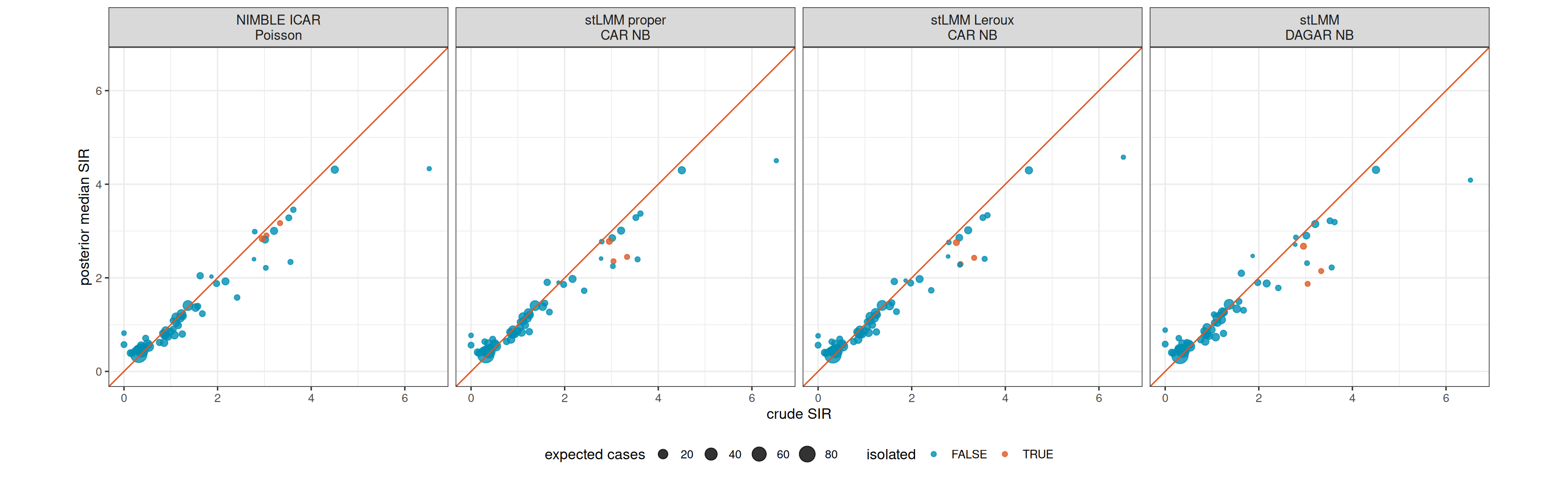
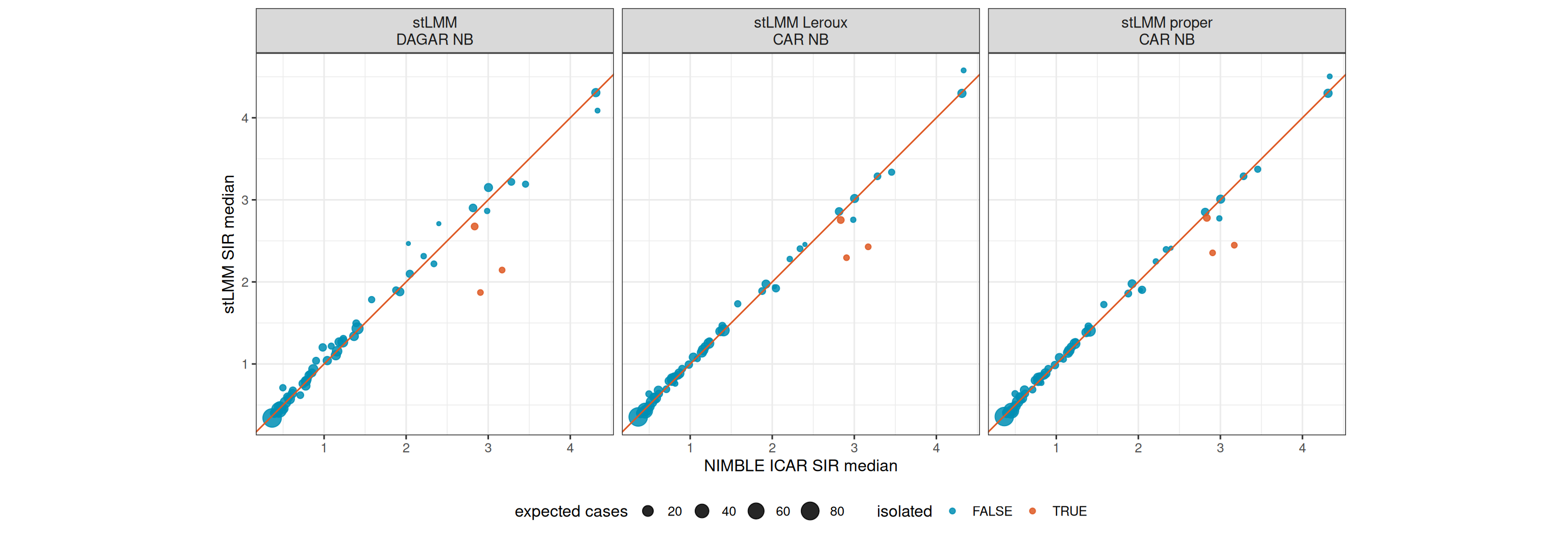
The table below compares posterior median SIR estimates from each stLMM fit against the NIMBLE ICAR posterior median SIR estimates. Values close to correlation one, RMSE near zero, and mean difference near zero indicate close agreement with the NIMBLE reference fit.
Code
nimble_col <- paste0("sir_median_", model_nimble)
stlmm_models <- c(model_car, model_leroux, model_dagar)
stlmm_cols <- paste0("sir_median_", stlmm_models)

sir_pair <- all_sir |>
  select(area, NAME, model, sir_median, prob_sir_gt_1) |>
  pivot_wider(names_from = model, values_from = c(sir_median, prob_sir_gt_1)) |>
  left_join(
    data.frame(
      area = ScotLip$area,
      crudeSIR = ScotLip$crudeSIR,
      CANCER = ScotLip$CANCER,
      CEXP = ScotLip$CEXP,
      degree_nimble = spdep::card(wards_nb),
      component = nb_comp$comp.id
    ),
    by = "area"
  )

pair_summary <- data.frame(
  comparison = paste(stlmm_models, "minus", model_nimble),
  correlation = unname(vapply(stlmm_cols, function(col)
    cor(sir_pair[[nimble_col]], sir_pair[[col]]), numeric(1))),
  rmse = unname(vapply(stlmm_cols, function(col)
    sqrt(mean((sir_pair[[col]] - sir_pair[[nimble_col]])^2)), numeric(1))),
  mean_difference = unname(vapply(stlmm_cols, function(col)
    mean(sir_pair[[col]] - sir_pair[[nimble_col]]), numeric(1)))
)

pair_summary |>
  mutate(across(where(is.numeric), ~ round(.x, 3))) |>
  knitr::kable(caption = "Pairwise SIR comparison against the NIMBLE ICAR fit.")
Pairwise SIR comparison against the NIMBLE ICAR fit.
| stLMM proper CAR NB minus NIMBLE ICAR Poisson |
0.992 |
0.136 |
-0.015 |
| stLMM Leroux CAR NB minus NIMBLE ICAR Poisson |
0.991 |
0.145 |
-0.012 |
| stLMM DAGAR NB minus NIMBLE ICAR Poisson |
0.977 |
0.227 |
-0.010 |
Maps and Scatter Plots
Code
ggplot(diagnostic_sir, aes(crudeSIR, sir_median)) +
  geom_point(aes(size = CEXP, color = degree_nimble == 0), alpha = 0.8) +
  geom_abline(intercept = 0, slope = 1, color = stlmm_color("secondary")) +
  facet_wrap(~ model, nrow = 1, labeller = as_labeller(panel_labels)) +
  coord_equal(xlim = c(0, 6.6), ylim = c(0, 6.6)) +
  scale_color_manual(values = c("FALSE" = stlmm_color("primary"), "TRUE" = stlmm_color("secondary"))) +
  labs(x = "crude SIR", y = "posterior median SIR", color = "isolated", size = "expected cases") +
  theme(strip.text = element_text(size = 11, lineheight = 0.95), legend.position = "bottom")
Code
nimble_stlmm_long <- bind_rows(lapply(seq_along(stlmm_models), function(j) {
  data.frame(
    area = sir_pair$area,
    NAME = sir_pair$NAME,
    CEXP = sir_pair$CEXP,
    degree_nimble = sir_pair$degree_nimble,
    model = stlmm_models[j],
    nimble_sir = sir_pair[[nimble_col]],
    stlmm_sir = sir_pair[[stlmm_cols[j]]]
  )
}))

ggplot(nimble_stlmm_long, aes(nimble_sir, stlmm_sir)) +
  geom_point(aes(size = CEXP, color = degree_nimble == 0), alpha = 0.85) +
  geom_abline(intercept = 0, slope = 1, color = stlmm_color("secondary")) +
  facet_wrap(~ model, nrow = 1, labeller = as_labeller(panel_labels)) +
  coord_equal() +
  scale_color_manual(values = c("FALSE" = stlmm_color("primary"), "TRUE" = stlmm_color("secondary"))) +
  labs(x = "NIMBLE ICAR SIR median", y = "stLMM SIR median",
       color = "isolated", size = "expected cases") +
  theme(strip.text = element_text(size = 11, lineheight = 0.95), legend.position = "bottom")
Posterior Quantile Comparisons
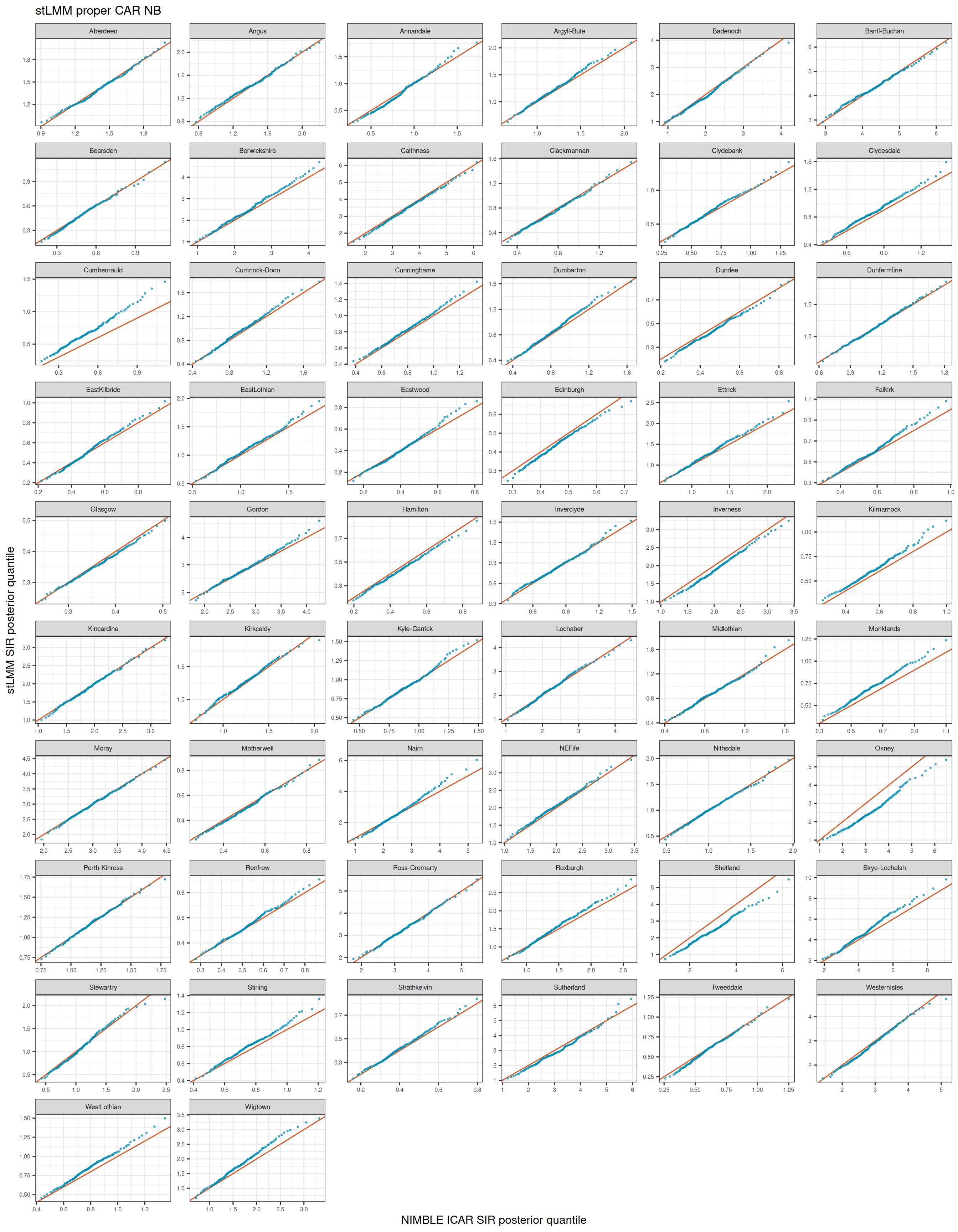
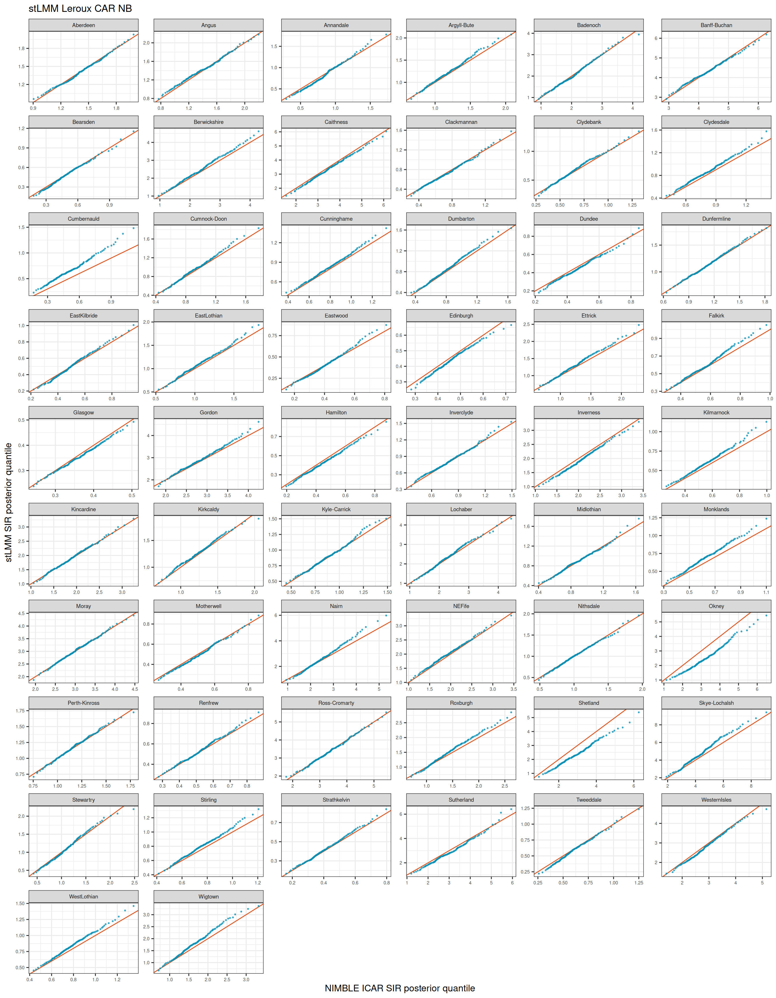
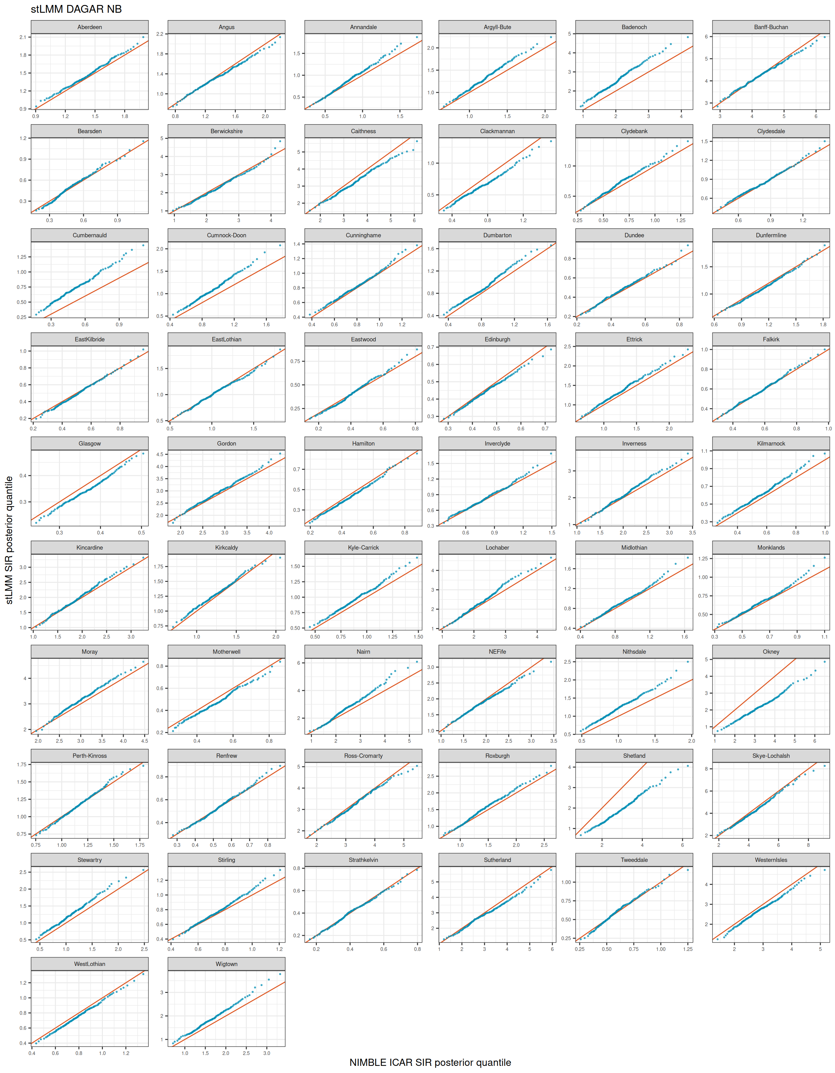
The median comparisons above show how closely the centers of the posterior SIR distributions align across areas. A fuller comparison also checks whether the posterior tails are similar. The Q-Q plots below compare matched posterior SIR quantiles from the NIMBLE ICAR fit and each stLMM fit for every county, one stLMM model at a time. These panels are meant as a broad diagnostic scan: points near the one-to-one line indicate similar posterior distributions for that county, while curvature or separated endpoints indicate differences in posterior spread or tail behavior.
Code
all_qq_dat <- make_qq_dat(ScotLip$area)

for (model_i in stlmm_models) {
  p <- ggplot(filter(all_qq_dat, model == model_i), aes(nimble, stlmm)) +
    geom_abline(intercept = 0, slope = 1, color = stlmm_color("secondary")) +
    geom_point(size = 0.45, alpha = 0.65, color = stlmm_color("primary")) +
    facet_wrap(~ NAME, scales = "free", ncol = 6) +
    labs(
      title = model_i,
      x = "NIMBLE ICAR SIR posterior quantile",
      y = "stLMM SIR posterior quantile"
    ) +
    theme(
      strip.text = element_text(size = 7),
      plot.title = element_text(size = 13),
      axis.text = element_text(size = 6)
    )

  print(p)
}
The Q-Q panels suggest that the stLMM posterior SIR distributions are broadly similar to the NIMBLE ICAR posterior distributions for many counties, especially in the center of the distributions. Departures are most visible where the point clouds bend away from the one-to-one line or separate in the upper tails. Those differences are expected to be more apparent than median differences because the models use different likelihoods, graph structures, and spatial prior forms.
Interpreting the Differences
The pairwise table, scatter plots, and Q-Q plots above compare complementary parts of the posterior SIR estimates. The median summaries show agreement in posterior center across all areas. The Q-Q plots show whether the county-level posterior distributions have similar spread and tail behavior.
The most important modeling differences are:
-
Likelihood: NIMBLE uses exact Poisson; stLMM uses large-size NB-PG. With
size = 1000, this is usually a small likelihood difference for these counts, but it is not zero.
-
Prior propriety and constraint: NIMBLE’s ICAR is improper and constrained with
zero_mean = 1; stLMM’s proper CAR, Leroux CAR, and DAGAR priors are proper and unconstrained.
-
Graph: NIMBLE uses a disconnected
poly2nb() graph with isolated regions; stLMM uses a connected graph with nearest-neighbor bridges.
-
Areal prior form: NIMBLE’s ICAR is the limiting intrinsic model. stLMM’s proper CAR uses \(\mathbf{D}-\rho\mathbf{G}\) with sampled \(\rho < 1\), Leroux CAR uses \((1-\rho)\mathbf{I}+\rho(\mathbf{D}-\mathbf{G})\), and DAGAR uses an ordered directed precision \(\mathbf{Q}_{\operatorname{DAGAR}}\).
-
Hyperpriors: NIMBLE uses a gamma prior on ICAR precision; stLMM uses a half-\(t\) prior on the process standard deviation and a bounded prior on \(\rho\).