Purpose
This article compares stLMM with lme4 for models with independent grouped random effects. The goal is comparison, not replacement. lme4 is an expansive, mature, and widely used mixed-model package. Bates et al. (2015) describe lme4 as a modular system for fitting linear and generalized linear mixed models using sparse-matrix methods and profiled likelihood or REML estimation.
There are several important things lme4 can do that stLMM currently cannot:
- estimate covariance among random-effect terms, as in
(1 + x | group);
- fit nested and crossed random-effect structures through the standard formula interface;
- fit models by ML or REML and report likelihood-based diagnostics;
- support a broad GLMM workflow through
glmer().
The fair comparison is narrower. We compare models with fixed effects, one or more independent group-level random effects, and likelihoods that both packages can represent exactly or approximately. In stLMM, a random intercept and two independent random slopes are written as
y ~ x1 + x2 + iid(group) + x1:iid(group) + x2:iid(group)
The matching lme4 formula is
y ~ x1 + x2 + (1 | group) + (0 + x1 | group) + (0 + x2 | group)
For numeric random-effect terms, this is also equivalent to the compact lme4 formula
y ~ x1 + x2 + (1 + x1 + x2 || group)
This intentionally avoids (1 + x1 + x2 | group), because that model estimates the covariance matrix among group-level intercepts and slopes.
The non-Gaussian comparisons need extra caution:
-
stLMM uses Pólya-Gamma data augmentation for binomial and negative-binomial likelihoods;
-
lme4::glmer() fits GLMMs by likelihood approximation;
-
stLMM represents Poisson models through a large-size negative-binomial approximation, not a native Poisson likelihood;
-
stLMM currently fixes the negative-binomial size parameter, while lme4::glmer.nb() estimates it.
Show helper functions
posterior_means <- function(fit, burn = 500L){
  draws <- as_samples(fit, burn = burn, metadata = FALSE)
  draws$.chain <- NULL
  draws$.iteration <- NULL
  vapply(draws, mean, numeric(1))
}

posterior_sds <- function(fit, burn = 500L){
  draws <- as_samples(fit, burn = burn, metadata = FALSE)
  draws$.chain <- NULL
  draws$.iteration <- NULL
  vapply(draws, sd, numeric(1))
}

round_numeric_columns <- function(x, digits = 3){
  is_num <- vapply(x, is.numeric, logical(1))
  x[is_num] <- lapply(x[is_num], round, digits = digits)
  x
}

format_estimate_with_uncertainty <- function(estimate, uncertainty, digits = 3){
  paste0(
    format(round(estimate, digits), nsmall = digits),
    " (",
    format(round(uncertainty, digits), nsmall = digits),
    ")"
  )
}

fixed_effect_table <- function(st_fit, lme4_fit, truth, burn = 500L){
  st_mean <- posterior_means(st_fit, burn = burn)
  st_sd <- posterior_sds(st_fit, burn = burn)
  lme4_beta <- fixef(lme4_fit)
  lme4_se <- sqrt(diag(vcov(lme4_fit)))

  data.frame(
    parameter = names(lme4_beta),
    truth = unname(truth[names(lme4_beta)]),
    stLMM = format_estimate_with_uncertainty(
      unname(st_mean[names(lme4_beta)]),
      unname(st_sd[names(lme4_beta)])
    ),
    lme4 = format_estimate_with_uncertainty(
      unname(lme4_beta),
      unname(lme4_se[names(lme4_beta)])
    ),
    difference = unname(st_mean[names(lme4_beta)] - lme4_beta),
    row.names = NULL
  )
}

diagnostic_table <- function(st_fit, parameters, burn = 500L){
  s <- summary(st_fit, burn = burn)
  s$diagnostics[parameters, c("parameter", "rhat", "effective_size"),
                drop = FALSE]
}

iid_random_effect_compare <- function(st_fit, lme4_fit, st_term = 1L,
                                      lme4_column = "(Intercept)",
                                      burn = 500L){
  st_mean <- posterior_means(st_fit, burn = burn)
  prefix <- paste0("iid_", st_term, "_")
  st_re <- st_mean[grep(paste0("^", prefix), names(st_mean))]
  names(st_re) <- sub(paste0("^", prefix), "", names(st_re))

  lme4_re <- ranef(lme4_fit)$group[[lme4_column]]
  names(lme4_re) <- rownames(ranef(lme4_fit)$group)

  common <- intersect(names(st_re), names(lme4_re))
  data.frame(
    group = common,
    stLMM = unname(st_re[common]),
    lme4 = unname(lme4_re[common])
  )
}
Gaussian Models
Gaussian mixed models are the cleanest comparison because both packages target the same linear mixed-model likelihood for independent random effects.
Simple Data
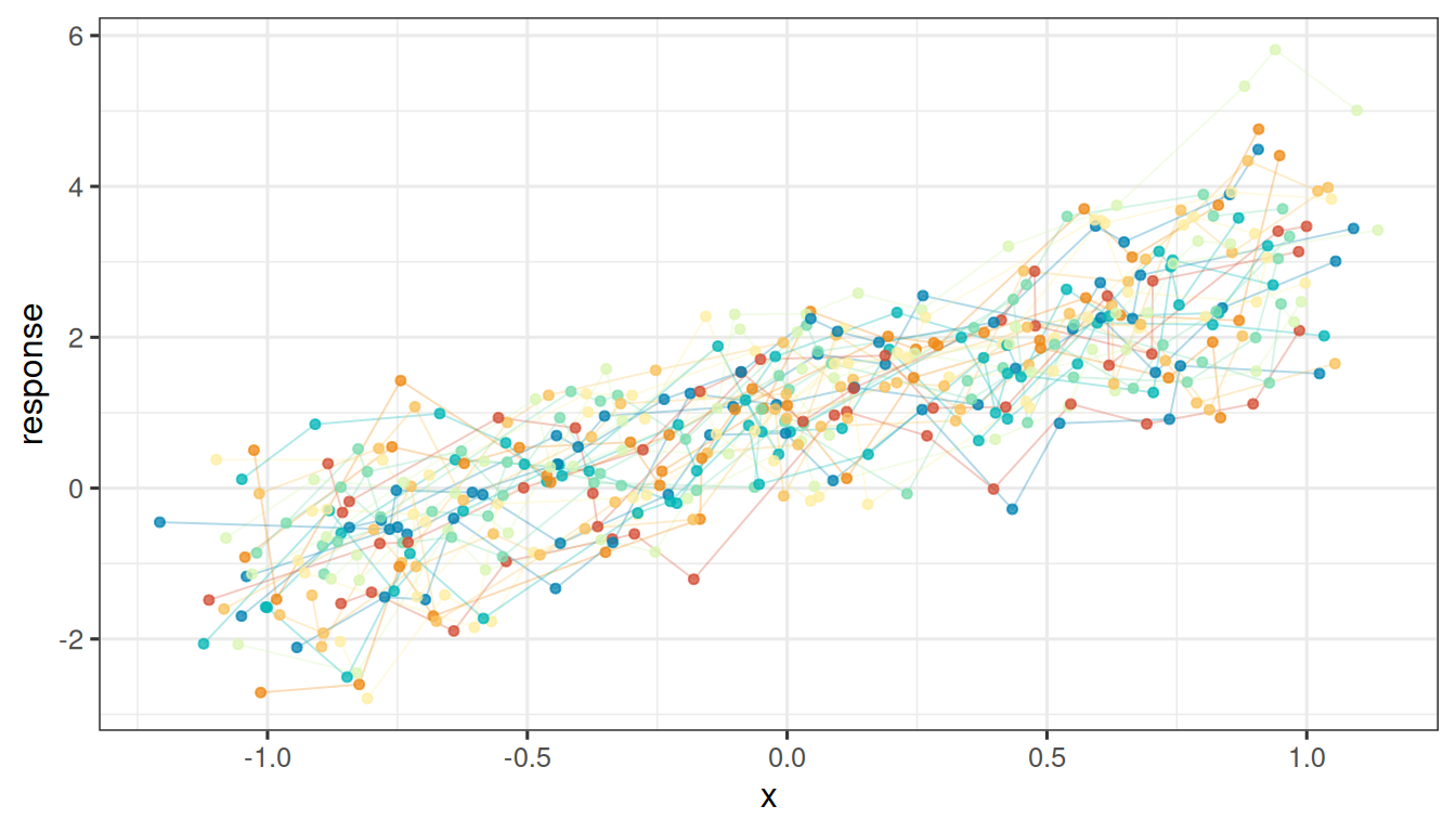
Each group has its own intercept and its own slope for x, and those two group-level effects are independent in the data-generating model.
Show simulation code
simulate_gaussian_slope_data <- function(seed = 1,
                                         n_group = 30,
                                         n_per_group = 15,
                                         beta = c("(Intercept)" = 1, x = 2),
                                         sigma_intercept = 0.5,
                                         sigma_slope = 0.5,
                                         tau = 0.5){
  set.seed(seed)

  group <- factor(rep(sprintf("g%02d", seq_len(n_group)),
                      each = n_per_group))
  x <- rep(seq(-1, 1, length.out = n_per_group), n_group) +
    rnorm(n_group * n_per_group, sd = 0.08)

  alpha_intercept <- rnorm(n_group, sd = sigma_intercept)
  alpha_slope <- rnorm(n_group, sd = sigma_slope)
  names(alpha_intercept) <- levels(group)
  names(alpha_slope) <- levels(group)

  mu <- beta[["(Intercept)"]] + beta[["x"]] * x +
    alpha_intercept[group] + alpha_slope[group] * x

  data.frame(
    y = mu + rnorm(length(mu), sd = tau),
    x = x,
    group = group
  )
}

gauss_dat <- simulate_gaussian_slope_data(seed = 1)
gauss_true_beta <- c("(Intercept)" = 1, x = 2)
gauss_true_sd <- c(
  residual = 0.5,
  `random intercept` = 0.5,
  `random slope x` = 0.5
)
The simulated dataset has 30 groups with 15 observations in each group.
Fits
The stLMM fit uses weak inverse-gamma priors for the Gaussian residual variance and the two independent iid random-effect variances. Posterior inference is based on three chains, with \(\hat R\) diagnostics reported below. The lme4 fit uses REML.
Code
gauss_st_time <- system.time({
  gauss_st <- stLMM(
    y ~ x + iid(group) + x:iid(group),
    data = gauss_dat,
    priors = list(
      resid = list(tau_sq = ig(2, 0.5)),
      iid_1 = list(sigma_sq = ig(2, 0.5)),
      iid_2 = list(sigma_sq = ig(2, 0.5))
    ),
    n_samples = 1500,
    chains = 3,
    verbose = FALSE
  )
})

gauss_lme4_time <- system.time({
  gauss_lme4 <- lmer(
    y ~ x + (1 | group) + (0 + x | group),
    data = gauss_dat,
    REML = TRUE
  )
})
Parameter Estimates
Fixed-effect values are shown as estimate followed by uncertainty in parentheses. For stLMM, the parenthetical value is posterior SD; for lme4, it is the fixed-effect SE reported by summary().
The random-effect standard-deviation table reports point estimates only. Those variance-component summaries are useful for comparing scale across packages.
Show table code
gauss_st_mean <- posterior_means(gauss_st, burn = 500)
gauss_lme4_vc <- as.data.frame(VarCorr(gauss_lme4))
gauss_lme4_vc <- gauss_lme4_vc[gauss_lme4_vc$grp != "Residual", ,
                               drop = FALSE]

gauss_beta_tab <- fixed_effect_table(
  gauss_st, gauss_lme4, truth = gauss_true_beta, burn = 500
)
gauss_sd_tab <- data.frame(
  component = names(gauss_true_sd),
  truth = unname(gauss_true_sd),
  stLMM = c(
    sqrt(gauss_st_mean[["tau_sq"]]),
    sqrt(gauss_st_mean[["iid_1_sigma_sq"]]),
    sqrt(gauss_st_mean[["iid_2_sigma_sq"]])
  ),
  lme4 = c(sigma(gauss_lme4), gauss_lme4_vc$sdcor),
  row.names = NULL
)
gauss_sd_tab$difference <- gauss_sd_tab$stLMM - gauss_sd_tab$lme4
gauss_diag <- diagnostic_table(
  gauss_st,
  parameters = c("(Intercept)", "x", "tau_sq",
                 "iid_1_sigma_sq", "iid_2_sigma_sq"),
  burn = 500
)

knitr::kable(round_numeric_columns(gauss_beta_tab, 3))
| (Intercept) |
1 |
1.001 (0.103) |
0.991 (0.095) |
0.010 |
| x |
2 |
2.068 (0.122) |
2.074 (0.124) |
-0.006 |
Show table code
knitr::kable(round_numeric_columns(gauss_sd_tab, 3))
| residual |
0.5 |
0.536 |
0.535 |
0.001 |
| random intercept |
0.5 |
0.519 |
0.504 |
0.015 |
| random slope x |
0.5 |
0.641 |
0.639 |
0.002 |
Show table code
knitr::kable(round_numeric_columns(gauss_diag, 3))
| (Intercept) |
(Intercept) |
1.008 |
100.044 |
| x |
x |
1.038 |
225.668 |
| tau_sq |
tau_sq |
1.010 |
485.638 |
| iid_1_sigma_sq |
iid_1_sigma_sq |
1.001 |
1760.118 |
| iid_2_sigma_sq |
iid_2_sigma_sq |
1.000 |
2038.608 |
Show plotting code
gauss_re <- rbind(
  cbind(term = "intercept",
        iid_random_effect_compare(gauss_st, gauss_lme4, st_term = 1,
                                  lme4_column = "(Intercept)", burn = 500)),
  cbind(term = "slope x",
        iid_random_effect_compare(gauss_st, gauss_lme4, st_term = 2,
                                  lme4_column = "x", burn = 500))
)

ggplot(gauss_re, aes(lme4, stLMM)) +
  geom_abline(slope = 1, intercept = 0, color = "grey45", linewidth = 0.4) +
  geom_point(size = 1.8, alpha = 0.85, color = stlmm_color("primary")) +
  facet_wrap(~ term, scales = "free") +
  labs(
    x = "lme4 conditional mode",
    y = "stLMM posterior mean"
  )
Logistic Mixed Model
The logistic comparison uses Bernoulli responses with a logit link and an independent group random intercept.
Show logistic simulation code
simulate_logistic_data <- function(seed = 1,
                                   n_group = 30,
                                   n_per_group = 12,
                                   beta = c("(Intercept)" = -0.5, x = 1),
                                   sigma_intercept = 0.5){
  set.seed(seed)

  group <- factor(rep(sprintf("g%02d", seq_len(n_group)),
                      each = n_per_group))
  x <- rnorm(n_group * n_per_group)
  alpha <- rnorm(n_group, sd = sigma_intercept)
  names(alpha) <- levels(group)
  eta <- beta[["(Intercept)"]] + beta[["x"]] * x + alpha[group]

  data.frame(
    y = rbinom(length(eta), size = 1, prob = plogis(eta)),
    x = x,
    group = group
  )
}

logit_dat <- simulate_logistic_data(seed = 1)
logit_truth <- c("(Intercept)" = -0.5, x = 1)
logit_sigma <- 0.5
Code
logit_st_time <- system.time({
  logit_st <- stLMM(
    y ~ x + iid(group),
    data = logit_dat,
    family = "binomial",
    priors = list(iid_1 = list(sigma_sq = ig(2, 0.5))),
    n_samples = 1000,
    chains = 3,
    verbose = FALSE
  )
})

logit_lme4_time <- system.time({
  logit_lme4 <- glmer(
    y ~ x + (1 | group),
    data = logit_dat,
    family = binomial,
    nAGQ = 1
  )
})
Show logistic table code
logit_st_mean <- posterior_means(logit_st, burn = 500)
logit_vc <- as.data.frame(VarCorr(logit_lme4))
logit_vc <- logit_vc[logit_vc$grp != "Residual", , drop = FALSE]
logit_beta_tab <- fixed_effect_table(
  logit_st, logit_lme4, truth = logit_truth, burn = 500
)
logit_sd_tab <- data.frame(
  component = "random intercept",
  truth = logit_sigma,
  stLMM = sqrt(logit_st_mean[["iid_1_sigma_sq"]]),
  lme4 = logit_vc$sdcor[1],
  difference = sqrt(logit_st_mean[["iid_1_sigma_sq"]]) - logit_vc$sdcor[1]
)
logit_diag <- diagnostic_table(
  logit_st,
  parameters = c("(Intercept)", "x", "iid_1_sigma_sq"),
  burn = 500
)

knitr::kable(round_numeric_columns(logit_beta_tab, 3))
| (Intercept) |
-0.5 |
-0.607 (0.157) |
-0.600 (0.142) |
-0.008 |
| x |
1.0 |
0.936 (0.141) |
0.918 (0.144) |
0.017 |
Show logistic table code
knitr::kable(round_numeric_columns(logit_sd_tab, 3))
| random intercept |
0.5 |
0.508 |
0.385 |
0.122 |
Show logistic table code
knitr::kable(round_numeric_columns(logit_diag, 3))
| (Intercept) |
(Intercept) |
1.001 |
514.843 |
| x |
x |
1.002 |
772.534 |
| iid_1_sigma_sq |
iid_1_sigma_sq |
1.010 |
234.639 |
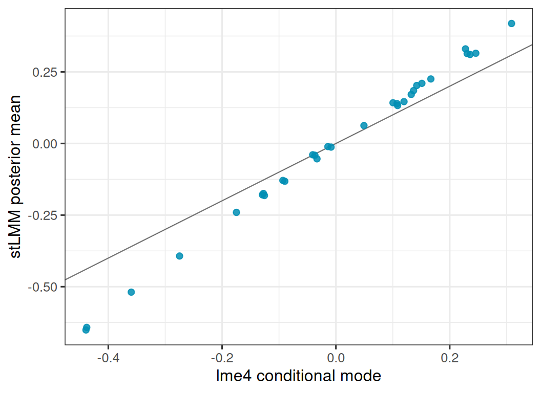
In this simulation, the fixed-effect estimates are close across packages. The random-intercept standard deviation is closer to the simulated truth under stLMM than under lme4. The scatter plot below shows the same pattern in the group-level conditional modes: they are strongly associated, but the points are not centered exactly on the 1:1 line because the estimated random-intercept scale differs between the two fits.
Show plotting code
logit_re <- iid_random_effect_compare(logit_st, logit_lme4, burn = 500)

ggplot(logit_re, aes(lme4, stLMM)) +
  geom_abline(slope = 1, intercept = 0, color = "grey45", linewidth = 0.4) +
  geom_point(size = 1.8, alpha = 0.85, color = stlmm_color("primary")) +
  labs(
    x = "lme4 conditional mode",
    y = "stLMM posterior mean"
  )
Poisson Data and the NB Approximation
stLMM does not currently fit a native Poisson likelihood. The package can fit a negative-binomial model with large fixed size, where
\[
\operatorname{var}(y_i) = \mu_i + \frac{\mu_i^2}{r},
\]
and this approaches the Poisson variance as the size \(r\) becomes large. This is an approximation check, not an exact likelihood comparison. We use size = 1000. This large size can mix more slowly, so this section uses longer chains than the logistic example.
Show Poisson simulation code
simulate_poisson_data <- function(seed = 1,
                                  n_group = 30,
                                  n_per_group = 12,
                                  beta = c("(Intercept)" = 0.5, x = 0.5),
                                  sigma_intercept = 0.5){
  set.seed(seed)

  group <- factor(rep(sprintf("g%02d", seq_len(n_group)),
                      each = n_per_group))
  x <- rnorm(n_group * n_per_group)
  alpha <- rnorm(n_group, sd = sigma_intercept)
  names(alpha) <- levels(group)
  eta <- beta[["(Intercept)"]] + beta[["x"]] * x + alpha[group]

  data.frame(
    y = rpois(length(eta), lambda = exp(eta)),
    x = x,
    group = group
  )
}

poisson_dat <- simulate_poisson_data(seed = 1)
poisson_truth <- c("(Intercept)" = 0.5, x = 0.5)
poisson_sigma <- 0.5
poisson_approx_size <- 1000
Code
poisson_st_time <- system.time({
  poisson_st <- stLMM(
    y ~ x + iid(group),
    data = poisson_dat,
    family = "negative_binomial",
    size = poisson_approx_size,
    priors = list(iid_1 = list(sigma_sq = ig(2, 0.5))),
    n_samples = 5000,
    chains = 3,
    verbose = FALSE
  )
})

poisson_lme4_time <- system.time({
  poisson_lme4 <- glmer(
    y ~ x + (1 | group),
    data = poisson_dat,
    family = poisson
  )
})
Show Poisson-approximation table code
poisson_st_mean <- posterior_means(poisson_st, burn = 2500)
poisson_vc <- as.data.frame(VarCorr(poisson_lme4))
poisson_vc <- poisson_vc[poisson_vc$grp != "Residual", , drop = FALSE]
poisson_beta_tab <- fixed_effect_table(
  poisson_st, poisson_lme4, truth = poisson_truth, burn = 2500
)
poisson_sd_tab <- data.frame(
  component = "random intercept",
  truth = poisson_sigma,
  stLMM = sqrt(poisson_st_mean[["iid_1_sigma_sq"]]),
  lme4 = poisson_vc$sdcor[1],
  difference = sqrt(poisson_st_mean[["iid_1_sigma_sq"]]) - poisson_vc$sdcor[1]
)
poisson_diag <- diagnostic_table(
  poisson_st,
  parameters = c("(Intercept)", "x", "iid_1_sigma_sq"),
  burn = 2500
)

knitr::kable(round_numeric_columns(poisson_beta_tab, 3))
| (Intercept) |
0.5 |
0.350 (0.108) |
0.379 (0.112) |
-0.029 |
| x |
0.5 |
0.497 (0.042) |
0.495 (0.042) |
0.003 |
Show Poisson-approximation table code
knitr::kable(round_numeric_columns(poisson_sd_tab, 3))
| random intercept |
0.5 |
0.58 |
0.555 |
0.025 |
Show Poisson-approximation table code
knitr::kable(round_numeric_columns(poisson_diag, 3))
| (Intercept) |
(Intercept) |
1.109 |
17.278 |
| x |
x |
1.016 |
90.277 |
| iid_1_sigma_sq |
iid_1_sigma_sq |
1.020 |
192.937 |
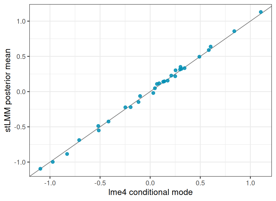
The Poisson approximation recovers the fixed effects reasonably well. The diagnostics also show that this large-size NB approximation gives a more challenging posterior computation than the logistic model. The intercept \(\hat R\) remains above the usual target even after the longer run, so this section should be read as both an estimator comparison and a caution about using the current approximation as a stand-in for a native Poisson likelihood.
Show plotting code
poisson_re <- iid_random_effect_compare(poisson_st, poisson_lme4, burn = 2500)

ggplot(poisson_re, aes(lme4, stLMM)) +
  geom_abline(slope = 1, intercept = 0, color = "grey45", linewidth = 0.4) +
  geom_point(size = 1.8, alpha = 0.85, color = stlmm_color("primary")) +
  labs(
    x = "lme4 conditional mode",
    y = "stLMM posterior mean"
  )
Negative-Binomial Mixed Model
The final example simulates negative-binomial counts with fixed size 3. The stLMM fit uses this known fixed size. The lme4::glmer.nb() fit estimates the size parameter, so this is close but not exactly the same estimation problem. Estimating the negative-binomial size parameter in stLMM would make this comparison cleaner and is a natural future extension.
Show negative-binomial simulation code
simulate_nb_data <- function(seed = 1,
                             n_group = 40,
                             n_per_group = 12,
                             beta = c("(Intercept)" = 0.5, x = 0.5),
                             sigma_intercept = 0.5,
                             size = 3){
  set.seed(seed)

  group <- factor(rep(sprintf("g%02d", seq_len(n_group)),
                      each = n_per_group))
  x <- rnorm(n_group * n_per_group)
  alpha <- rnorm(n_group, sd = sigma_intercept)
  names(alpha) <- levels(group)
  eta <- beta[["(Intercept)"]] + beta[["x"]] * x + alpha[group]

  data.frame(
    y = rnbinom(length(eta), size = size, mu = exp(eta)),
    x = x,
    group = group
  )
}

nb_size <- 3
nb_dat <- simulate_nb_data(seed = 1, size = nb_size)
nb_truth <- c("(Intercept)" = 0.5, x = 0.5)
nb_sigma <- 0.5
Code
nb_st_time <- system.time({
  nb_st <- stLMM(
    y ~ x + iid(group),
    data = nb_dat,
    family = "negative_binomial",
    size = nb_size,
    priors = list(iid_1 = list(sigma_sq = ig(2, 0.5))),
    n_samples = 1000,
    chains = 3,
    verbose = FALSE
  )
})

nb_lme4_time <- system.time({
  nb_lme4 <- glmer.nb(
    y ~ x + (1 | group),
    data = nb_dat
  )
})

nb_lme4_size <- getME(nb_lme4, "glmer.nb.theta")
Show negative-binomial table code
nb_st_mean <- posterior_means(nb_st, burn = 500)
nb_vc <- as.data.frame(VarCorr(nb_lme4))
nb_vc <- nb_vc[nb_vc$grp != "Residual", , drop = FALSE]
nb_beta_tab <- fixed_effect_table(
  nb_st, nb_lme4, truth = nb_truth, burn = 500
)
nb_sd_tab <- data.frame(
  component = "random intercept",
  truth = nb_sigma,
  stLMM = sqrt(nb_st_mean[["iid_1_sigma_sq"]]),
  lme4 = nb_vc$sdcor[1],
  difference = sqrt(nb_st_mean[["iid_1_sigma_sq"]]) - nb_vc$sdcor[1]
)
nb_size_tab <- data.frame(
  parameter = "negative-binomial size",
  truth = nb_size,
  stLMM = nb_size,
  lme4 = nb_lme4_size
)
nb_diag <- diagnostic_table(
  nb_st,
  parameters = c("(Intercept)", "x", "iid_1_sigma_sq"),
  burn = 500
)

knitr::kable(round_numeric_columns(nb_beta_tab, 3))
| (Intercept) |
0.5 |
0.382 (0.124) |
0.376 (0.131) |
0.006 |
| x |
0.5 |
0.540 (0.047) |
0.536 (0.046) |
0.003 |
Show negative-binomial table code
knitr::kable(round_numeric_columns(nb_sd_tab, 3))
| random intercept |
0.5 |
0.769 |
0.764 |
0.005 |
Show negative-binomial table code
knitr::kable(round_numeric_columns(nb_size_tab, 3))
| negative-binomial size |
3 |
3 |
3.423 |
Show negative-binomial table code
knitr::kable(round_numeric_columns(nb_diag, 3))
| (Intercept) |
(Intercept) |
1.019 |
94.873 |
| x |
x |
1.000 |
855.367 |
| iid_1_sigma_sq |
iid_1_sigma_sq |
1.000 |
826.891 |
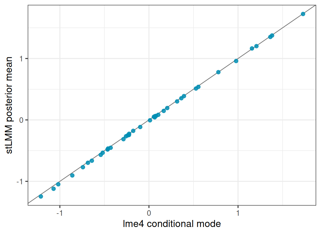
The negative-binomial fixed effects and random-intercept scale are close across the two packages, even though the comparison is not perfectly matched.
Show plotting code
nb_re <- iid_random_effect_compare(nb_st, nb_lme4, burn = 500)

ggplot(nb_re, aes(lme4, stLMM)) +
  geom_abline(slope = 1, intercept = 0, color = "grey45", linewidth = 0.4) +
  geom_point(size = 1.8, alpha = 0.85, color = stlmm_color("primary")) +
  labs(
    x = "lme4 conditional mode",
    y = "stLMM posterior mean"
  )
Runtime Summary
The runtime table records elapsed time for the fitted models above. The stLMM timings are for posterior sampling, while the lme4 timings are likelihood or REML fits. These are different computational targets.
Show runtime table code
runtime_tab <- data.frame(
  example = c(
    "Gaussian simple", "Gaussian simple",
    "logistic", "logistic",
    "Poisson approximation", "Poisson approximation",
    "negative binomial", "negative binomial"
  ),
  package = rep(c("stLMM", "lme4"), times = 4),
  task = c(
    "3 chains x 1500 posterior draws", "REML fit",
    "3 chains x 1000 posterior draws", "glmer binomial",
    "3 chains x 5000 posterior draws", "glmer Poisson",
    "3 chains x 1000 posterior draws", "glmer.nb"
  ),
  elapsed_seconds = c(
    gauss_st_time[["elapsed"]],
    gauss_lme4_time[["elapsed"]],
    logit_st_time[["elapsed"]],
    logit_lme4_time[["elapsed"]],
    poisson_st_time[["elapsed"]],
    poisson_lme4_time[["elapsed"]],
    nb_st_time[["elapsed"]],
    nb_lme4_time[["elapsed"]]
  )
)

knitr::kable(round_numeric_columns(runtime_tab, 3))
| Gaussian simple |
stLMM |
3 chains x 1500 posterior draws |
0.390 |
| Gaussian simple |
lme4 |
REML fit |
0.039 |
| logistic |
stLMM |
3 chains x 1000 posterior draws |
1.260 |
| logistic |
lme4 |
glmer binomial |
0.064 |
| Poisson approximation |
stLMM |
3 chains x 5000 posterior draws |
5.734 |
| Poisson approximation |
lme4 |
glmer Poisson |
0.061 |
| negative binomial |
stLMM |
3 chains x 1000 posterior draws |
92.758 |
| negative binomial |
lme4 |
glmer.nb |
0.872 |
Takeaways
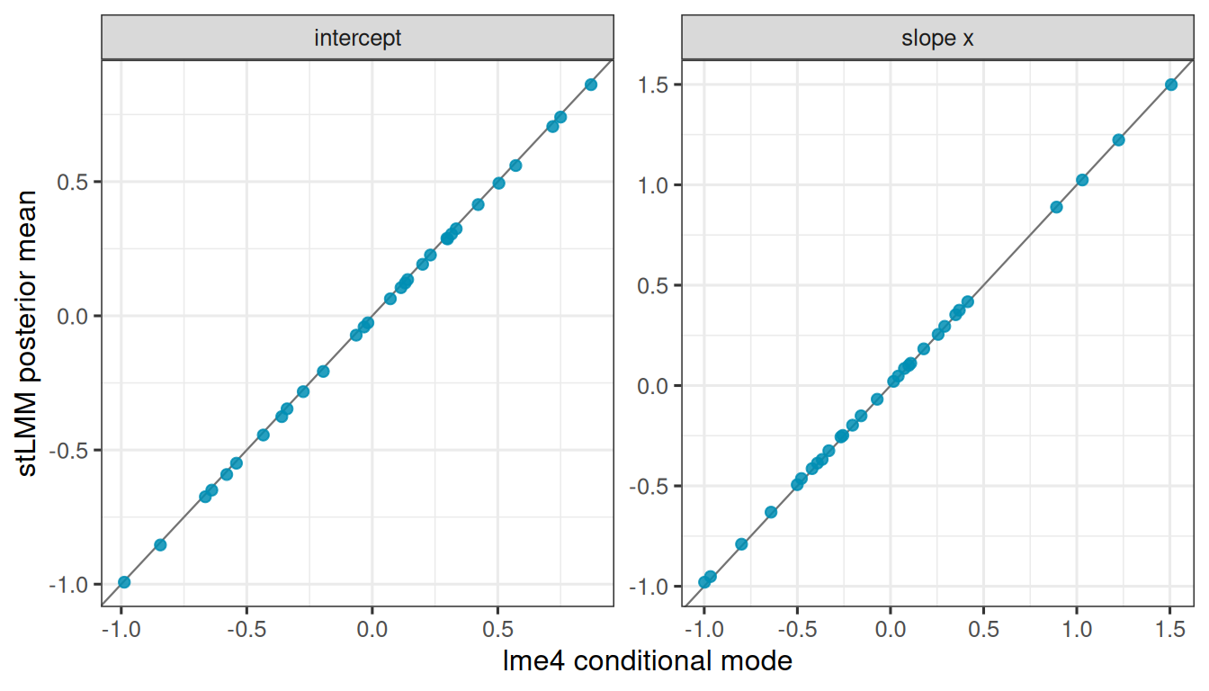
For Gaussian models with independent grouped random effects, stLMM and lme4 produce very similar fixed effects, variance components, and group-level effects in this simulation.
The logistic comparison is the cleanest GLMM comparison. The Poisson example shows that a large-size negative-binomial fit can track a native Poisson glmer() fit for fixed effects, but it also shows that the approximation can require more posterior simulation effort. The negative-binomial example is useful, but the packages treat the size parameter differently: fixed in stLMM, estimated in lme4. A native Poisson likelihood and an estimated negative-binomial size parameter would both make future comparisons more direct.
Bates, Douglas, Martin Maechler, Ben Bolker, and Steve Walker. 2015.
“Fitting Linear Mixed-Effects Models Using lme4.” Journal of Statistical Software 67 (1): 1–48.
https://doi.org/10.18637/jss.v067.i01.