
Probit models with stLMM
Binary mixed models, Albert-Chib augmentation, and prediction
Source:vignettes/a15-probit-models.qmd
1 Overview
This vignette introduces binary probit models in stLMM. The example uses a binary response, a structured AR(1) latent time effect, fitted probabilities, retained time-effect draws, and holdout prediction. Probit models use the same formula grammar as Gaussian and logistic models, but the response must be binary 0/1 and the probability scale is defined through the standard normal cdf.
Use family = "probit" for the native probit likelihood. For compatibility with familiar R model syntax, family = binomial(link = "probit") is also accepted and dispatches to the same probit sampler.
2 Probit model
For binary responses, stLMM uses a probit mixed model. The response can be viewed as a binomial response with one trial,
\[ y_i \mid p_i \sim \operatorname{Binomial}(1, p_i), \]
with linear predictor
\[ \eta_i = \Phi^{-1}(p_i). \]
For the time-structured example below,
\[ \eta_i = \beta_0 + x_i\beta_1 + w_{t_i}, \qquad \mathbf{w} = \{w_1,\ldots,w_T\}^\top \sim N\{\mathbf{0}, \sigma_w^2\mathbf{R}(\phi)\}. \]
The probability is
\[ p_i = \Phi(\eta_i), \]
where \(\Phi(\cdot)\) is the standard normal cdf.
This notation maps directly to the package outputs. For probit models, fitted(..., scale = "link") returns posterior summaries of \(\eta_i\), while the default scale = "response" returns posterior summaries of \(p_i\). Similarly, predict(..., scale = "link") returns prediction samples on the linear predictor scale, and the default response scale returns predicted probabilities. If y_samples = TRUE, prediction simulates binary outcomes.
3 Albert-Chib updates
The probit sampler uses the Albert-Chib latent-normal representation (Albert and Chib 1993). Introduce a latent utility
\[ z_i = \eta_i + \epsilon_i, \qquad \epsilon_i \sim N(0, 1), \]
and observe
\[ y_i = 1(z_i > 0). \]
Conditional on the current linear predictor, \(z_i\) is sampled from a normal distribution truncated above or below zero according to the observed binary response. Conditional on the sampled latent utilities, the model is Gaussian with unit observation precision. This lets stLMM reuse the same collapsed structured-process machinery used by Gaussian models.
There is no residual variance parameter tau_sq in a probit model. The unit latent variance identifies the probit scale, so tau_sq priors, starting values, tuning values, and the Gaussian resid() term are not used with family = "probit".
For structured process terms such as ar1(), nngp(), car(), or car_time(), the process is collapsed during parameter updates. In probit structured-process models, stLMM() saves the in-chain process draws by default as save_process = list(start = 1, thin = 1) because those draws are already needed for the Albert-Chib augmentation. Calling recover() selects from these saved draws for fitted values and prediction. Users can thin the retained process grid with save_process = list(start = ..., thin = ...), or set save_process = FALSE when only parameter samples are needed.
4 Simulated binary time series
We simulate repeated binary observations over a shared time index. The latent AR(1) process creates temporal dependence in the probability of response after accounting for the fixed effect. We hold out a subset of rows throughout the time range by setting y = NA; these rows do not contribute to the likelihood, but their covariates and time values are retained for prediction.
Code
n_time <- 34
n_per_time <- 12

time <- rep(seq_len(n_time), each = n_per_time)
x <- rnorm(n_time * n_per_time)

beta <- c("(Intercept)" = -0.15, x = 0.75)
sigma_w_sq <- 0.85^2
phi <- 0.75
time_support <- seq_len(n_time)
w <- rmvnorm(
  mean = rep(0, n_time),
  Sigma = sigma_w_sq * ar1_cor(time_support, phi = phi)
)

eta <- beta["(Intercept)"] + beta["x"] * x + w[time]
prob <- pnorm(eta)
y <- rbinom(length(prob), size = 1, prob = prob)

holdout <- logical(length(y))
holdout_id <- unlist(tapply(seq_along(y), time, function(z) sample(z, 2)))
holdout[holdout_id] <- TRUE

dat <- data.frame(
  y = y,
  x = x,
  time = time,
  prob_true = prob
)
dat$y[holdout] <- NA
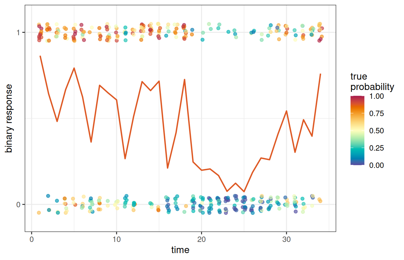
The exploratory plot shows the complete simulated binary dataset before the holdout values are hidden from the model. Points are jittered vertically so repeated zeros and ones remain visible. The line shows the time-specific mean of the true simulated probabilities.
Show plotting code
plot_dat <- dat
plot_dat$y_full <- y

prob_by_time <- aggregate(prob_true ~ time, data = plot_dat, FUN = mean)

ggplot(plot_dat, aes(time, y_full)) +
  geom_jitter(
    aes(color = prob_true),
    width = 0.18,
    height = 0.05,
    alpha = 0.65,
    size = 1.6
  ) +
  geom_line(
    data = prob_by_time,
    aes(y = prob_true),
    color = stlmm_color("secondary"),
    linewidth = 0.8
  ) +
  scale_color_gradientn(
    colors = stlmm_palette(),
    limits = c(0, 1)
  ) +
  scale_y_continuous(
    breaks = c(0, 1),
    limits = c(-0.1, 1.1)
  ) +
  labs(
    x = "time",
    y = "binary response",
    color = "true\nprobability"
  )
5 Fit
The family = "probit" argument selects the binary probit likelihood. Unlike the logistic binomial likelihood, there is no trials argument because this implementation expects binary 0/1 responses.
Code
fit <- stLMM(
  y ~ x + ar1(time),
  data = dat,
  family = "probit",
  priors = list(
    beta = normal(mean = 0, sd = 3),
    ar1_1 = list(
      sigma_sq = half_t(df = 3, scale = 1),
      phi = uniform(0.05, 0.95)
    )
  ),
  starting = list(ar1_1 = list(sigma_sq = 0.5, phi = 0.5)),
  tuning = list(ar1_1 = list(sigma_sq = 0.05, phi = 0.1)),
  n_samples = 1000,
  verbose = FALSE
)

summary(fit)
stLMM summary
formula: y ~ x + ar1(time)
observations: 408 (340 observed, 68 missing response)
posterior draws: 1000
family: probit
fixed effects: 2
grouped random-effect coefficients: 0
process terms: 1
residual variance: global tau_sq
beta:
mean sd q2.5 q50.0 q97.5
(Intercept) -0.0233 0.4353 -0.7793 -0.0510 1.0366
x 0.7476 0.1003 0.5599 0.7448 0.9565
sigma_sq:
mean sd q2.5 q50.0 q97.5
ar1_1_sigma_sq 0.9368 0.5917 0.3827 0.7991 2.5115
theta:
mean sd q2.5 q50.0 q97.5
ar1_1_phi 0.6214 0.1865 0.2456 0.6322 0.9391The fixed effects use a weakly informative normal prior. The AR(1) term has a prior on its process variance and temporal association parameter. Notice that no tau_sq prior is supplied.
6 Latent process recovery
Structured process terms are integrated out during parameter updates. For this Albert-Chib model, the sampler has already saved the in-chain AR(1) process draws needed for augmentation. Calling recover() selects and labels the retained latent time effects; it does not run a separate post-fit latent-normal reconstruction chain. The recovered AR(1) effects line up with the sorted fitted time support.
Binary data provide less direct information about the latent process scale than Gaussian responses, so the process variance posterior can remain broad. The simulation below uses a moderately strong time effect so the recovered process pattern is visible in a short example run.
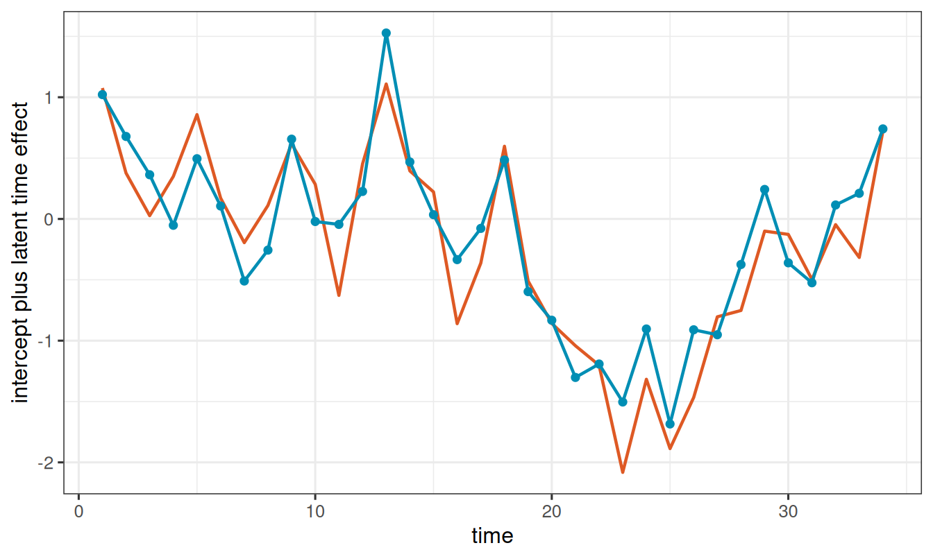
The process mean and the fixed intercept can trade a nearly constant shift in a finite MCMC run. For that reason, the plot below compares the intercept-plus-process contribution, \(\beta_0 + w_t\), rather than \(w_t\) alone.
Code
rec <- recover(fit, sub_sample = list(start = 301, thin = 2))
rec_draws <- as_samples(rec, include_w = TRUE, metadata = FALSE)
w_cols <- paste0("w_ar1_1_", seq_along(time_support))
intercept_w_samples <- sweep(
  as.matrix(rec_draws[, w_cols, drop = FALSE]),
  1,
  rec_draws[["(Intercept)"]],
  "+"
)

w_summary <- data.frame(
  time = time_support,
  truth = beta["(Intercept)"] + w,
  posterior_mean = colMeans(intercept_w_samples)
)

head(w_summary)
time truth posterior_mean
w_ar1_1_1 1 1.0755473 1.02164397
w_ar1_1_2 2 0.3769890 0.67773163
w_ar1_1_3 3 0.0270054 0.36316412
w_ar1_1_4 4 0.3496245 -0.05212063
w_ar1_1_5 5 0.8570904 0.49484910
w_ar1_1_6 6 0.1712200 0.10625044In the plot, the orange line is the true simulated intercept-plus-process contribution and the blue line is the posterior mean estimate.
Show plotting code
ggplot(w_summary, aes(time)) +
  geom_line(
    aes(y = truth),
    color = stlmm_color("secondary"),
    linewidth = 0.8
  ) +
  geom_line(
    aes(y = posterior_mean),
    color = stlmm_color("primary"),
    linewidth = 0.8
  ) +
  geom_point(
    aes(y = posterior_mean),
    color = stlmm_color("primary"),
    size = 1.6
  ) +
  labs(
    x = "time",
    y = "intercept plus latent time effect"
  )
7 Fitted probabilities
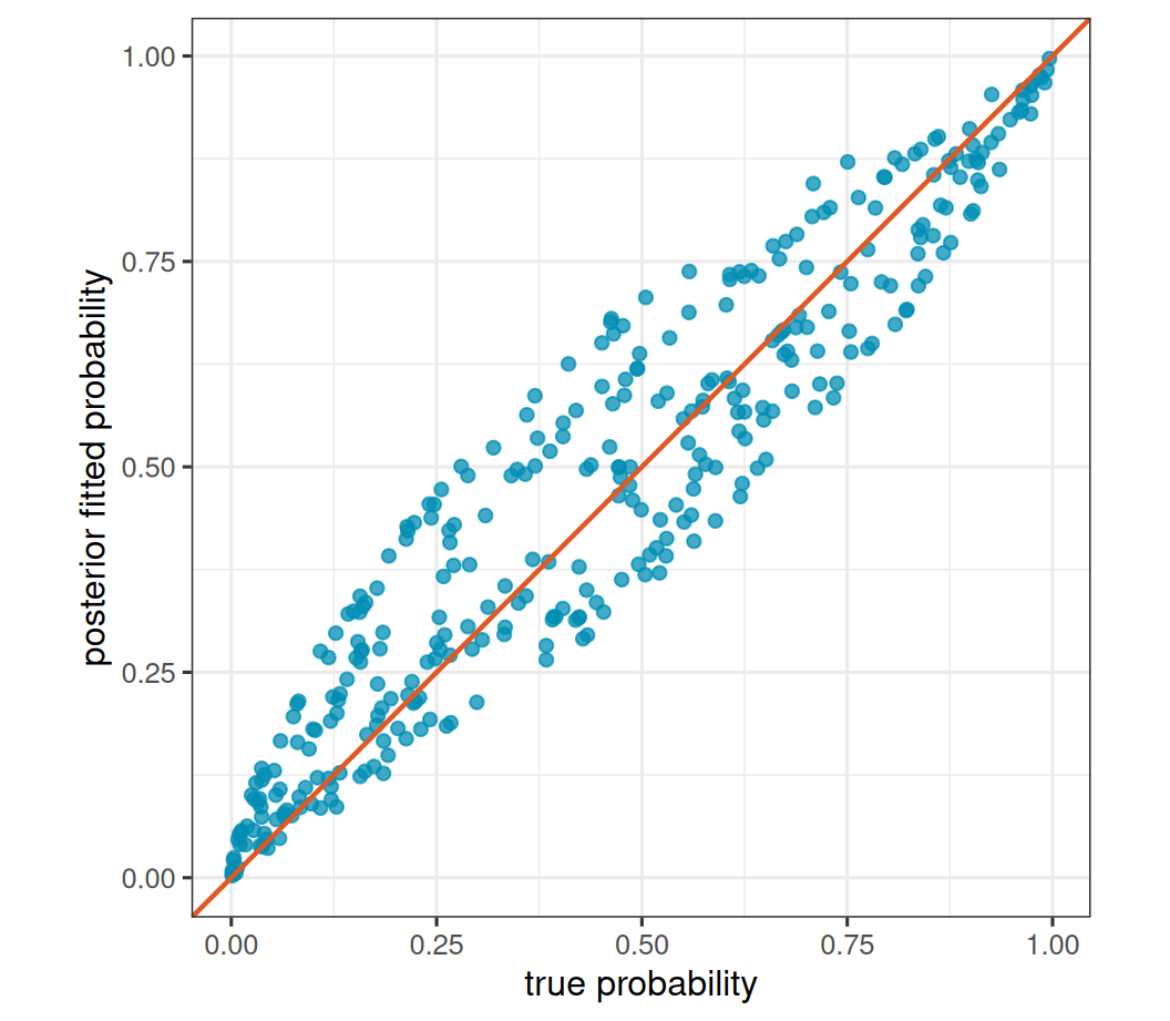
By default, fitted() returns posterior fitted probabilities for probit models. Because this model has a structured AR(1) term, fitted values need latent process draws. For this Albert-Chib fit those draws were saved during MCMC; here we use the recovered object so the fitted values line up with the same selected draw grid used above.
Code
fitted_prob <- fitted(rec)

fitted_link <- fitted(
  rec,
  scale = "link"
)

head(data.frame(probability = fitted_prob, link = fitted_link))
probability link
1 0.6891091 0.5477090
2 0.8525355 1.1605768
3 0.6367332 0.3894608
4 0.9764973 2.2285315
5 0.8741785 1.2709285
6 0.6406312 0.4009300The two scales are related by the standard normal cdf. For example, pnorm(fitted_link) is on the probability scale, up to the difference between transforming posterior means and averaging transformed posterior draws.
Show plotting code
fitted_dat <- data.frame(
  truth = dat$prob_true[!holdout],
  fitted = fitted_prob[!holdout]
)
fitted_lim <- range(fitted_dat$truth, fitted_dat$fitted)

ggplot(fitted_dat, aes(truth, fitted)) +
  geom_point(
    color = stlmm_color("primary"),
    alpha = 0.75,
    size = 1.8
  ) +
  geom_abline(
    intercept = 0,
    slope = 1,
    color = stlmm_color("secondary"),
    linewidth = 0.8
  ) +
  coord_equal(
    xlim = fitted_lim,
    ylim = fitted_lim
  ) +
  labs(
    x = "true probability",
    y = "posterior fitted probability"
  )
8 Holdout prediction
Prediction rows for this model need the fixed-effect covariates and the fitted time value. Here all prediction rows are held-out observations on the fitted time support. The call below uses the fitted object directly to show that probit process predictions can use the saved in-chain process draws without first creating a recovery object.
Code
stLMM prediction
  mean samples: 350 draws x 68 rows
  newdata: TRUE
  joint: FALSE
  y samples: simulated
  process samples: ar1_1
The mu_samples matrix contains predicted probabilities by default. The y_samples matrix contains posterior predictive binary draws. The full prediction summary has one row for each prediction row, so here we print only the first few rows.
Code
pred_summary <- summary(pred)
pred_draws <- as_samples(pred, sample = "all", metadata = FALSE)
mu_cols <- paste0("mu_", seq_len(nrow(holdout_new)))
y_cols <- paste0("y_", seq_len(nrow(holdout_new)))
pred_prob <- colMeans(pred_draws[, mu_cols, drop = FALSE])
pred_y <- colMeans(pred_draws[, y_cols, drop = FALSE])

prediction_summary <- data.frame(
  time = holdout_new$time,
  truth_prob = dat$prob_true[holdout],
  predicted_prob = pred_prob,
  observed_y = y[holdout],
  predicted_y_mean = pred_y
)

head(prediction_summary)
time truth_prob predicted_prob observed_y predicted_y_mean
mu_1 1 0.9884570 0.9764973 1 0.9714286
mu_2 1 0.8013648 0.7622365 1 0.7857143
mu_3 2 0.8888978 0.9218124 1 0.9057143
mu_4 2 0.6343094 0.7257864 1 0.7314286
mu_5 3 0.4642067 0.5918422 0 0.6400000
mu_6 3 0.8522230 0.9023426 1 0.9200000Code
head(pred_summary$mu) mean sd q2.5 q50.0 q97.5
4 0.9764973 0.02849939 0.9014306 0.9864107 0.9994070
10 0.7622365 0.13112499 0.4740137 0.7802191 0.9575402
15 0.9218124 0.05848262 0.7591932 0.9380690 0.9910345
16 0.7257864 0.12222691 0.4707236 0.7432309 0.9254312
27 0.5918422 0.13146721 0.3285229 0.6043670 0.8098184
31 0.9023426 0.06741801 0.7405585 0.9221419 0.9816919Code
head(pred_summary$y) mean sd q2.5 q50.0 q97.5
4 0.9714286 0.1668371 0 1 1
10 0.7857143 0.4109133 0 1 1
15 0.9057143 0.2926442 0 1 1
16 0.7314286 0.4438510 0 1 1
27 0.6400000 0.4806872 0 1 1
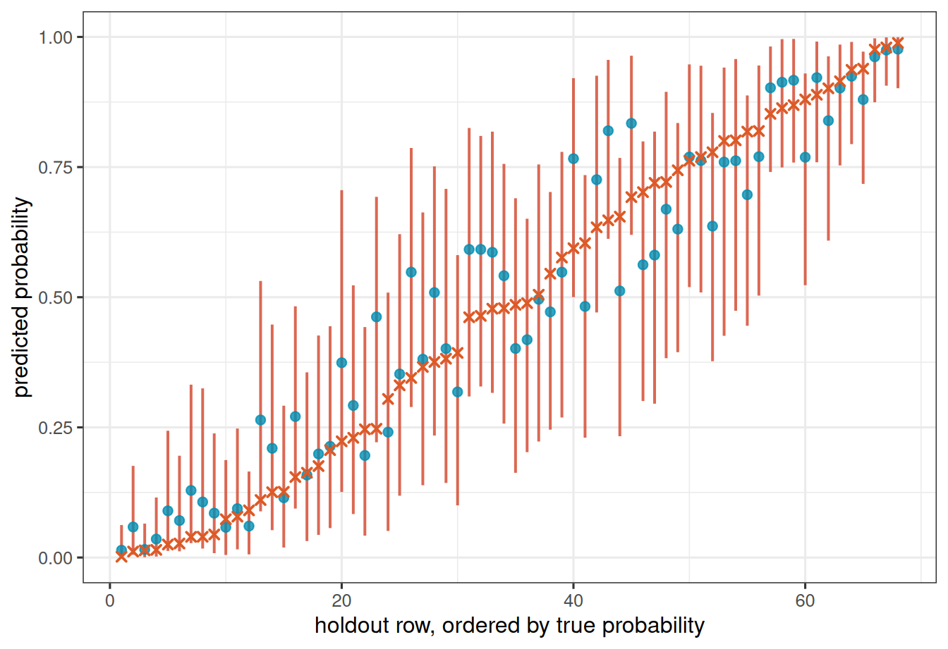
31 0.9200000 0.2716816 0 1 1The holdout plot compares the true simulated probabilities, which are known here because this is a simulation, with the posterior predicted probabilities. The blue points are posterior means, the vertical lines are 95% credible intervals for \(p_i\), and the orange crosses are the true simulated probabilities.
Show plotting code
plot_pred <- prediction_summary
plot_pred$mean <- pred_summary$mu[, "mean"]
plot_pred$q2.5 <- pred_summary$mu[, "q2.5"]
plot_pred$q97.5 <- pred_summary$mu[, "q97.5"]
plot_pred$row <- seq_len(nrow(plot_pred))
plot_pred <- plot_pred[order(plot_pred$truth_prob), ]
plot_pred$row <- seq_len(nrow(plot_pred))
interval_color <- stlmm_discrete_colors(4)[4]

ggplot(plot_pred, aes(row, mean)) +
  geom_linerange(
    aes(ymin = q2.5, ymax = q97.5),
    color = interval_color,
    alpha = 0.85,
    linewidth = 0.7
  ) +
  geom_point(
    color = stlmm_color("primary"),
    size = 2,
    alpha = 0.8
  ) +
  geom_point(
    aes(y = truth_prob),
    color = stlmm_color("secondary"),
    shape = 4,
    stroke = 1
  ) +
  labs(
    x = "holdout row, ordered by true probability",
    y = "predicted probability"
  )
9 What this example illustrates
Probit stLMM models use the same formula grammar as Gaussian and logistic models, but the response must be binary 0/1 and there is no tau_sq. Use family = "probit" or family = binomial(link = "probit").
For probit models, fitted and predicted means are probabilities on the response scale by default. Use scale = "link" to work with the linear predictor. If y_samples = TRUE, prediction simulates binary outcomes, not Gaussian residual noise.
The AR(1) effects in this example are retained during fitting and then selected by recover(). For Albert-Chib structured-process models, predict(fit, ...) can also use the saved process draws directly; recover() is useful when you want the usual recovery object or a narrower retained draw grid. This differs from Gaussian process and CAR examples, where recover() draws the process values post hoc.