Skip to contents
Show setup
library(tidyverse)
library(sf)
library(Matrix)
library(stLMM)
library(RhpcBLASctl)

colville_data_dir <- "colville_data"

source(file.path(colville_data_dir, "utils.R"))
source(file.path(colville_data_dir, "article-cache.R"))

article_id <- "colville-stlmm-vignette"

set.seed(1)
theme_set(theme_bw(base_size = 12))

1 Overview

This capstone closes the Washington biomass series by moving from county-year summaries of the simplified agb_live_mg_ha response to a forestland-support analysis for a user-defined area in Washington, the Colville National Forest. May and Finley (2025) modeled aboveground biomass density with a semi-continuous space-time response distribution. The response has a point mass at zero and positive continuous support otherwise. Their model has two linked pieces: a binary model for the zero/nonzero part of the response and a Gaussian model for biomass magnitude conditional on being in the nonzero component. In this article, the binary indicator is defined using FIA forest-condition status, so the resulting estimates are tied to FIA’s forested definition.

The inferential target in this reanalysis differs in a mild way from May and Finley (2025). Here, a plot’s Bernoulli response is 1 if any condition on that plot is forested. May and Finley (2025) instead set the response to 1 if the plot had positive aboveground biomass; under that definition, a forested plot with zero observed biomass would contribute a zero to the binary model. The FIA-based definition used here more directly targets biomass density on forested land. Section Section 10 discusses possible extensions that would align the binary stage even more closely with FIA’s plot design and condition proportions.

Like the original analysis, posterior predictive draws from the two fitted models are multiplied draw-by-draw to form posterior predictive draws from the zero-inflated biomass distribution, \[ b^{(m)}(\mathbf{s}, t) = z^{(m)}(\mathbf{s}, t)\, y^{(m)}(\mathbf{s}, t), \tag{1}\] where \(z^{(m)}\) is a Bernoulli FIA-forested draw and \(y^{(m)}\) is a draw from the live biomass process on FIA-defined forested plots. This article follows that workflow for the portion of Colville National Forest in the Northern Cascades ecoregion.

In addition to this definitional difference for \(z\), the implementation differs from May and Finley (2025) in a few modeling details. The covariance function multi_res_sep_exp used in each model is a reparameterization of their two-scale separable exponential covariance, with an alpha weight for the broad and local components. The forested-plot biomass model also uses a square-root transformation rather than the cube-root transformation used for the North Cascades analysis in the paper. These choices keep the example aligned with FIA definitions while preserving the paper’s two-part posterior predictive product.

This article is reproducible from its Quarto source or extracted R code. The shared Colville data bundle is the only data download needed to run the article locally.

The aims are:

  1. Fit a space-time Bernoulli model for whether an FIA plot is forested under FIA definitions.
  2. Fit a space-time Gaussian model for live aboveground biomass density on FIA-defined forested plots.
  3. Predict both processes on annual grids for the full ecoregion and the National Forest from 1999 through 2026.
  4. Form draw-matched posterior predictive biomass draws by multiplying FIA-forested status and forested-plot biomass magnitude draws.
  5. Summarize the annual posterior predictive distribution for the National Forest.

The covariance model is multi_res_sep_exp, a two-scale sum of separable exponential space-time correlations. This is the stLMM analogue of the multi-scale covariance model emphasized by May and Finley (2025). Coordinates are modeled in kilometers so spatial decay parameters can be assigned interpretable priors.

2 Prepared data

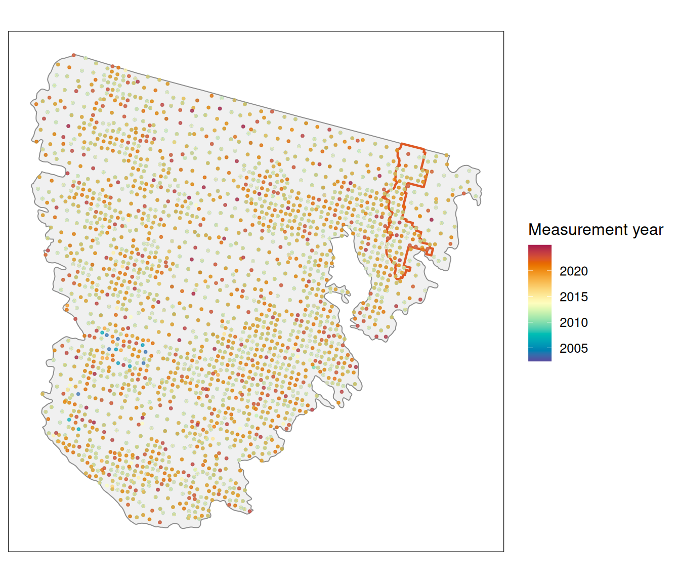
The data bundle expands to a directory named colville_data. Run the Quarto source or extracted R script from the directory that contains colville_data. The prepared spatial files are stored in the TCC CONUS Albers CRS. The model uses x_km and y_km, which are the same projected coordinates divided by 1000, and time, a decimal measurement year for FIA plots. The prediction supports are a 5 km grid over the Northern Cascades ecoregion and a 2 km grid over the Colville National Forest portion of that ecoregion.

Code
fia_plots <- st_read(file.path(colville_data_dir, "fia_plots_model_data.gpkg"),
                     layer = "fia_plots_model_data",
                     quiet = TRUE)

prediction_grid_eco <- st_read(file.path(colville_data_dir, "prediction_grid_eco_5km_1999_2026.gpkg"),
                               layer = "prediction_grid_eco_5km_1999_2026",
                               quiet = TRUE)

prediction_grid_nf <- st_read(file.path(colville_data_dir, "prediction_grid_nf_2km_1999_2026.gpkg"),
                              layer = "prediction_grid_nf_2km_1999_2026",
                              quiet = TRUE)

nf <- st_read(file.path(colville_data_dir, "colville_national_forest_northern_cascades.gpkg"),
              layer = "colville_national_forest_northern_cascades",
              quiet = TRUE)

eco <- st_read(file.path(colville_data_dir, "northern_cascades_ecoregion.gpkg"),
               layer = "northern_cascades_ecoregion",
               quiet = TRUE)

fia_dat <- fia_plots %>%
  st_drop_geometry() %>%
  mutate(
    forested = as.integer(forested)
  )

pred_eco_dat <- prediction_grid_eco %>%
  st_drop_geometry()

pred_nf_dat <- prediction_grid_nf %>%
  st_drop_geometry()

glimpse(fia_dat)
Rows: 4,701
Columns: 14
$ x             <dbl> -1913536, -1913509, -1897207, -1919670, -1897885, -19089…
$ y             <dbl> 3011706, 2983835, 2990277, 2994688, 2996117, 2988147, 29…
$ x_km          <dbl> -1913.536, -1913.509, -1897.207, -1919.670, -1897.885, -…
$ y_km          <dbl> 3011.706, 2983.835, 2990.277, 2994.688, 2996.117, 2988.1…
$ year          <int> 2002, 2002, 2002, 2002, 2002, 2002, 2002, 2002, 2002, 20…
$ time          <dbl> 2002.559, 2002.767, 2002.493, 2002.463, 2002.792, 2002.7…
$ invyr         <int> 2002, 2002, 2002, 2002, 2002, 2002, 2002, 2002, 2002, 20…
$ measyear      <int> 2002, 2002, 2002, 2002, 2002, 2002, 2002, 2002, 2002, 20…
$ measmon       <int> 7, 10, 6, 6, 10, 10, 8, 9, 10, 7, 6, 10, 8, 7, 10, 8, 10…
$ measday       <int> 24, 8, 30, 19, 17, 1, 6, 22, 16, 23, 30, 18, 5, 19, 14, …
$ meas_date     <date> 2002-07-24, 2002-10-08, 2002-06-30, 2002-06-19, 2002-10…
$ forested      <int> 1, 1, 0, 1, 1, 1, 1, 1, 1, 1, 0, 1, 1, 1, 1, 1, 0, 1, 1,…
$ biomass_Mg_ha <dbl> 39.07074, 432.96775, 0.00000, 104.59630, 112.19616, 34.7…
$ c_Mg_ha       <dbl> 18.73343, 218.50052, 0.00000, 52.07652, 55.64929, 16.867…
Code
glimpse(pred_eco_dat)
Rows: 32,424
Columns: 6
$ x    <dbl> -1882553, -1882553, -1882553, -1882553, -1882553, -1882553, -1882…
$ y    <dbl> 2934006, 2934006, 2934006, 2934006, 2934006, 2934006, 2934006, 29…
$ x_km <dbl> -1882.553, -1882.553, -1882.553, -1882.553, -1882.553, -1882.553,…
$ y_km <dbl> 2934.006, 2934.006, 2934.006, 2934.006, 2934.006, 2934.006, 2934.…
$ year <int> 1999, 2000, 2001, 2002, 2003, 2004, 2005, 2006, 2007, 2008, 2009,…
$ time <dbl> 1999, 2000, 2001, 2002, 2003, 2004, 2005, 2006, 2007, 2008, 2009,…

Code
glimpse(pred_nf_dat)
Rows: 4,508
Columns: 6
$ x    <dbl> -1763076, -1763076, -1763076, -1763076, -1763076, -1763076, -1763…
$ y    <dbl> 3049306, 3049306, 3049306, 3049306, 3049306, 3049306, 3049306, 30…
$ x_km <dbl> -1763.076, -1763.076, -1763.076, -1763.076, -1763.076, -1763.076,…
$ y_km <dbl> 3049.306, 3049.306, 3049.306, 3049.306, 3049.306, 3049.306, 3049.…
$ year <int> 1999, 2000, 2001, 2002, 2003, 2004, 2005, 2006, 2007, 2008, 2009,…
$ time <dbl> 1999, 2000, 2001, 2002, 2003, 2004, 2005, 2006, 2007, 2008, 2009,…
Code
ggplot() +
  geom_sf(data = eco, fill = "grey94", color = "grey55", linewidth = 0.35) +
  geom_sf(data = nf, fill = NA, color = stlmm_color("secondary"), linewidth = 0.8) +
  geom_sf(data = fia_plots, aes(color = time), size = 0.7, alpha = 0.7) +
  scale_color_gradientn(colors = stlmm_palette(), name = "Measurement year") +
  coord_sf(datum = NA) +
  labs(x = NULL, y = NULL)

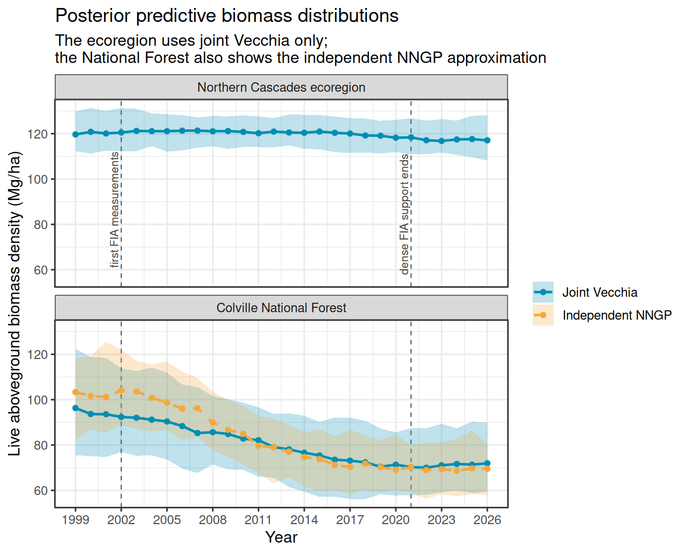
The prediction grids span 1999 through 2026, which is wider than the FIA measurement record available for this example. The table below makes this temporal support explicit. Measurements begin in 2002 and are fairly dense through 2021, then become sparse in the last few years. Keeping the full prediction period is useful pedagogically because it shows how the fitted space-time process borrows information across time: years before the first plot measurements and years after dense FIA support are informed by temporal dependence, spatial structure, and parameter uncertainty rather than by direct same-year observations.

Show plot-count table code
data_support_start <- min(fia_dat$year, na.rm = TRUE)
data_support_end <- max(fia_dat$year, na.rm = TRUE)
data_support_dense_end <- 2021
prediction_years <- sort(unique(pred_nf_dat$year))

plot_counts_by_year <- tibble(year = prediction_years) %>%
  left_join(
    fia_dat %>%
      group_by(year) %>%
      summarize(
        plots = n(),
        forested_plots = sum(forested == 1),
        .groups = "drop"
      ),
    by = "year"
  ) %>%
  mutate(across(c(plots, forested_plots), ~replace_na(.x, 0L))) %>%
  mutate(
    support = case_when(
      year < data_support_start ~ "no same-year FIA measurements",
      year == data_support_start ~ "first measurement year",
      year <= data_support_dense_end ~ "dense FIA support",
      year <= data_support_end ~ "sparse recent support",
      TRUE ~ "no same-year FIA measurements"
    )
  )

knitr::kable(
  plot_counts_by_year,
  caption = "FIA plot measurements by year in the Colville National Forest portion of the Northern Cascades ecoregion."
)
FIA plot measurements by year in the Colville National Forest portion of the Northern Cascades ecoregion.
year plots forested_plots support
1999 0 0 no same-year FIA measurements
2000 0 0 no same-year FIA measurements
2001 0 0 no same-year FIA measurements
2002 194 154 first measurement year
2003 230 197 dense FIA support
2004 207 167 dense FIA support
2005 248 207 dense FIA support
2006 208 179 dense FIA support
2007 215 183 dense FIA support
2008 194 155 dense FIA support
2009 260 193 dense FIA support
2010 224 179 dense FIA support
2011 234 186 dense FIA support
2012 228 186 dense FIA support
2013 197 154 dense FIA support
2014 235 196 dense FIA support
2015 230 188 dense FIA support
2016 228 197 dense FIA support
2017 206 179 dense FIA support
2018 224 178 dense FIA support
2019 229 181 dense FIA support
2020 222 181 dense FIA support
2021 210 168 dense FIA support
2022 174 128 sparse recent support
2023 76 66 sparse recent support
2024 28 18 sparse recent support
2025 0 0 no same-year FIA measurements
2026 0 0 no same-year FIA measurements

3 Model settings

stLMM parameterizes exponential correlations as exp(-phi * distance). If range_05 is the distance where correlation reaches 0.05, then phi = -log(0.05) / range_05. The broad component gets lower spatial decay and longer temporal persistence than the local component by using non-overlapping prior ranges.

Code
cor_at_range <- 0.05

decay_from_range <- function(range_05) {
  -log(cor_at_range) / range_05
}

## Broad process: approximately 25-100 km and 1-200 years.
phi_1_bounds <- decay_from_range(rev(c(25, 100)))
lambda_1_bounds <- decay_from_range(rev(c(1, 500)))

## Local process: approximately 1-25 km and 1-200 years.
phi_2_bounds <- decay_from_range(rev(c(1, 25)))
lambda_2_bounds <- decay_from_range(rev(c(1, 500)))

## Some chain thinning choices and metropolis controls for warmup.
n_chains <- 3
n_samples <- 2000
posterior_burn <- 1000
posterior_thin <- 10
prediction_draws_per_chain <- 25
prediction_thin <- ceiling((n_samples - posterior_burn) / prediction_draws_per_chain)
prediction_sub_sample <- list(start = posterior_burn + 1, thin = prediction_thin)
map_years <- c(1999, 2006, 2013, 2020, 2026)
n_report <- 1000

warmup_control <- list(
  batch_length = 25,
  min_batches = 10,
  max_batches = 20
)

## Request OpenMP threads for sampler and prediction work.
blas_set_num_threads(1)
n_omp_threads <- as.integer(Sys.getenv("STLMM_OMP_THREADS", unset = "4"))

## Space-time neighbor scaling for NNGP fitting and prediction. This treats one
## year as about 0.5 km when ordering nodes and finding neighbors.
fit_st_scale <- 0.5
pred_st_scale <- fit_st_scale

4 Bernoulli forest model

The Bernoulli model uses all FIA plot measurements. The response is forested, defined from FIA forest-condition status. This keeps the product estimate tied to FIA’s forested definition, while retaining the same two-part modeling structure.

The Bernoulli process variance is assigned a tight prior centered near 100 on the logit scale. With one Bernoulli trial per plot, this variance can be weakly identified: once fitted probabilities are close to zero or one, larger latent process variances have little effect on the likelihood. The tight prior regularizes this part of the model while still allowing substantial spatial-temporal variation in forest status.

Longer exploratory runs show good convergence for the model parameters. For this article, the code below uses starting values near those long-run posterior densities so shorter chains can run for the documentation build. To recreate the longer exploratory runs, use broader starting values and longer chains, for example n_samples = 20000.

Show starting value code
jitter_start <- function(value, amount = 0.02, bounds = NULL) {
  out <- rep(value, n_chains) * exp(rnorm(n_chains, 0, amount))

  if (!is.null(bounds)) {
    out <- pmin(pmax(out, bounds[1] + 1e-8), bounds[2] - 1e-8)
  }

  out
}
forest_fit <- stLMM(
  forested ~ nngp(x_km, y_km, time,
                  m = 15,
                  cov_model = "multi_res_sep_exp",
                  ordering = "maxmin",
                  st_scale = fit_st_scale),
  data = fia_dat,
  family = "binomial",
  starting = list(
    nngp_1 = list(
      sigma_sq = jitter_start(100),
      alpha = jitter_start(0.5, bounds = c(0, 1)),
      phi_1 = jitter_start(0.075, bounds = phi_1_bounds),
      lambda_1 = jitter_start(0.008, bounds = lambda_1_bounds),
      phi_2 = jitter_start(1.5, bounds = phi_2_bounds),
      lambda_2 = jitter_start(0.075, bounds = lambda_2_bounds)
    )
  ),
  priors = list(
    beta = normal(mean = 0, sd = 2),
    nngp_1 = list(
      sigma_sq = log_normal(meanlog = log(100), sdlog = 0.15),
      alpha = uniform(0, 1),
      phi_1 = uniform(phi_1_bounds[1], phi_1_bounds[2]),
      lambda_1 = uniform(lambda_1_bounds[1], lambda_1_bounds[2]),
      phi_2 = uniform(phi_2_bounds[1], phi_2_bounds[2]),
      lambda_2 = uniform(lambda_2_bounds[1], lambda_2_bounds[2])
    )
  ),
  n_samples = n_samples,
  chains = n_chains,
  warmup = warmup_control,
  save_process = prediction_sub_sample,
  n_omp_threads = n_omp_threads,
  n_report = n_report,
  verbose = TRUE
)

5 Forested-plot biomass model

Show biomass data code
biomass_dat <- fia_dat %>%
  filter(forested == 1) %>%
  mutate(biomass_sqrt = sqrt(biomass_Mg_ha))

The continuous model is fit to FIA-defined forested plot measurements. Following the paper’s general root-transformation strategy, this analysis models the square root of biomass density and then back-transforms prediction draws to Mg/ha.

biomass_fit <- stLMM(
  biomass_sqrt ~ nngp(x_km, y_km, time,
                          m = 15,
                          cov_model = "multi_res_sep_exp",
                          ordering = "maxmin",
                          st_scale = fit_st_scale),
  data = biomass_dat,
  family = "gaussian",
  starting = list(
    resid = list(
      tau_sq = jitter_start(1)
    ),
    nngp_1 = list(
      sigma_sq = jitter_start(45),
      alpha = jitter_start(0.5, bounds = c(0, 1)),
      phi_1 = jitter_start(0.05, bounds = phi_1_bounds),
      lambda_1 = jitter_start(0.01, bounds = lambda_1_bounds),
      phi_2 = jitter_start(2, bounds = phi_2_bounds),
      lambda_2 = jitter_start(0.01, bounds = lambda_2_bounds)
    )
  ),
  priors = list(
    beta = normal(mean = mean(biomass_dat$biomass_sqrt), sd = 5),
    resid = list(tau_sq = half_t(df = 3, scale = 1)),
    nngp_1 = list(
      sigma_sq = half_t(df = 3, scale = 2),
      alpha = uniform(0, 1),
      phi_1 = uniform(phi_1_bounds[1], phi_1_bounds[2]),
      lambda_1 = uniform(lambda_1_bounds[1], lambda_1_bounds[2]),
      phi_2 = uniform(phi_2_bounds[1], phi_2_bounds[2]),
      lambda_2 = uniform(lambda_2_bounds[1], lambda_2_bounds[2])
    )
  ),
  n_samples = n_samples,
  chains = n_chains,
  warmup = warmup_control,
  n_omp_threads = n_omp_threads,
  n_report = n_report,
  verbose = TRUE
)
Show fit summaries
forest_summary
stLMM multi-chain summary
  formula: forested ~ nngp(x_km, y_km, time, m = 15, cov_model = "multi_res_sep_exp", ordering = "maxmin", st_scale = fit_st_scale)
  chains: 3
  family: binomial
  observations: 4701
  posterior draws per chain: 2000 (1000 used after burn = 1000)
  process terms: 1

Parameters:
                    mean      sd     q2.5    q50.0    q97.5
(Intercept)       5.3391  1.3589   2.5283   5.4104   7.7649
nngp_1_sigma_sq 125.2697 12.3654 102.0247 125.6868 149.0125
nngp_1_alpha      0.5666  0.0713   0.4235   0.5677   0.6912
nngp_1_phi_1      0.0769  0.0189   0.0451   0.0756   0.1119
nngp_1_lambda_1   0.0070  0.0007   0.0061   0.0068   0.0089
nngp_1_phi_2      1.4729  0.6496   0.4839   1.4113   2.7048
nngp_1_lambda_2   0.0067  0.0006   0.0060   0.0065   0.0084

Chain diagnostics:
                      parameter   rhat effective_size
(Intercept)         (Intercept) 1.0239       430.0207
nngp_1_sigma_sq nngp_1_sigma_sq 1.1560        42.4904
nngp_1_alpha       nngp_1_alpha 1.0859        59.9900
nngp_1_phi_1       nngp_1_phi_1 1.1363        45.5626
nngp_1_lambda_1 nngp_1_lambda_1 1.0748        77.4525
nngp_1_phi_2       nngp_1_phi_2 1.0238        47.0345
nngp_1_lambda_2 nngp_1_lambda_2 1.0560       125.5167
Show fit summaries
biomass_summary
stLMM multi-chain summary
  formula: biomass_sqrt ~ nngp(x_km, y_km, time, m = 15, cov_model = "multi_res_sep_exp", ordering = "maxmin", st_scale = fit_st_scale)
  chains: 3
  family: gaussian
  observations: 3820
  posterior draws per chain: 2000 (1000 used after burn = 1000)
  process terms: 1

Parameters:
                   mean     sd    q2.5   q50.0   q97.5
(Intercept)      9.8833 0.7425  8.3422  9.9027 11.2738
tau_sq           0.5272 0.4638  0.0392  0.3498  1.5174
nngp_1_sigma_sq 37.7240 1.9584 34.2889 37.5013 41.9210
nngp_1_alpha     0.3825 0.0355  0.3226  0.3790  0.4573
nngp_1_phi_1     0.0390 0.0064  0.0307  0.0378  0.0560
nngp_1_lambda_1  0.0138 0.0026  0.0093  0.0137  0.0192
nngp_1_phi_2     2.2453 0.4914  1.2096  2.3122  2.9273
nngp_1_lambda_2  0.0126 0.0021  0.0082  0.0131  0.0158

Chain diagnostics:
                      parameter   rhat effective_size
(Intercept)         (Intercept) 1.0020      2348.2533
tau_sq                   tau_sq 1.2480        34.2773
nngp_1_sigma_sq nngp_1_sigma_sq 1.0525       125.2881
nngp_1_alpha       nngp_1_alpha 1.0086       119.1788
nngp_1_phi_1       nngp_1_phi_1 1.0432        17.2546
nngp_1_lambda_1 nngp_1_lambda_1 1.0245        84.0113
nngp_1_phi_2       nngp_1_phi_2 1.0285        36.3565
nngp_1_lambda_2 nngp_1_lambda_2 1.2229        38.1295

6 Fitted Covariance Summary

The fitted multi_res_sep_exp covariance has broad and local separable space-time components. The table below reports posterior median decay parameters in distance or time lag where correlation is approximately 0.05, using the same definition as the priors above.

Show summary code
posterior_medians <- function(fit) {
  samples <- as.matrix(as_mcmc(
    fit,
    burn = posterior_burn,
    thin = posterior_thin
  ))

  apply(samples, 2, stats::median)
}

param_value <- function(x, name) {
  unname(x[name])
}

forest_medians <- posterior_medians(forest_fit)
biomass_medians <- posterior_medians(biomass_fit)

practical_ranges <- function(p, model) {
  tibble(
    model = model,
    component = c("broad", "local"),
    spatial_range_km = -log(cor_at_range) / c(param_value(p, "nngp_1_phi_1"),
                                               param_value(p, "nngp_1_phi_2")),
    temporal_range_years = -log(cor_at_range) / c(param_value(p, "nngp_1_lambda_1"),
                                                  param_value(p, "nngp_1_lambda_2")),
    variance_weight = c(param_value(p, "nngp_1_alpha"),
                        1 - param_value(p, "nngp_1_alpha"))
  )
}

range_summary <- bind_rows(
  practical_ranges(forest_medians, "Forested probability"),
  practical_ranges(biomass_medians, "Forested-plot biomass")
) %>%
  mutate(across(where(is.numeric), ~ round(.x, 2)))

knitr::kable(
  range_summary,
  caption = "Posterior median practical ranges for the broad and local space-time covariance components."
)
Posterior median practical ranges for the broad and local space-time covariance components.
model component spatial_range_km temporal_range_years variance_weight
Forested probability broad 39.91 442.42 0.57
Forested probability local 2.17 460.28 0.43
Forested-plot biomass broad 79.68 217.29 0.38
Forested-plot biomass local 1.30 227.36 0.62

The Gaussian biomass model also has an observation-level residual variance, tau_sq, so its process variance can be compared with residual noise. The ratios below use posterior medians. The broad and local ratios allocate sigma_sq using the posterior median alpha and 1 - alpha.

Show summary code
sigma_sq <- param_value(biomass_medians, "nngp_1_sigma_sq")
alpha <- param_value(biomass_medians, "nngp_1_alpha")
tau_sq <- param_value(biomass_medians, "tau_sq")

signal_noise_summary <- tibble(
  component = c("total process", "broad component", "local component"),
  variance_ratio = c(sigma_sq / tau_sq,
                     alpha * sigma_sq / tau_sq,
                     (1 - alpha) * sigma_sq / tau_sq)
) %>%
  mutate(variance_ratio = round(variance_ratio, 2))

knitr::kable(
  signal_noise_summary,
  caption = "Posterior median biomass process-to-residual variance ratios."
)
Posterior median biomass process-to-residual variance ratios.
component variance_ratio
total process 109.00
broad component 41.29
local component 67.71

Ranges that are appreciable relative to the study area, temporal ranges that span multiple inventories, and process-to-residual variance ratios above one all indicate substantial spatial-temporal signal in the fitted biomass process.

7 Prediction

For the Gaussian model, recover() draws the latent process values before prediction. For the Bernoulli Pólya-Gamma model, recover() selects the saved in-chain process draws. The primary prediction calls below use Vecchia-style joint prediction for new NNGP nodes. We also compute independent NNGP predictions for the Colville National Forest grid to compare with the approximation used in May and Finley (2025).

With independent prediction, each new prediction node is conditionally simulated from the observed latent process and parameters without preserving residual dependence among new prediction nodes. That approximation is fast and reproduces the paper’s Figure 7 uncertainty summaries closely, including the narrower interval bands shown there. Here the joint prediction is the preferred summary when the final target is the posterior predictive distribution for an area average over many prediction cells. For area averages, preserving dependence among nearby prediction cells gives a more coherent posterior predictive distribution for the aggregate quantity. The tradeoff is computational: joint Vecchia prediction is slower and requires choosing an ordering and neighbor set for the prediction nodes.

The st_scale value affects only NNGP and Vecchia ordering and neighbor search, not the fitted covariance function. The paper used spatial range priors centered near 50 km for the ecosystem-scale component and 10 km for the local component, with temporal range priors centered near 100 years. Setting fit_st_scale = pred_st_scale = 0.5 treats one year of temporal separation as about 0.5 km when building the fitting and prediction neighbor sets. This gives a deliberate space-time exchange rate while preserving the original kilometer and year coordinates for covariance evaluation. For joint Vecchia prediction, we use max-min ordering because it gives a more space-filling ordering of the regular space-time prediction lattice than coordinate sorting.

Show prediction helper code
predict_support_joint <- function(pred_dat) {
  list(
    forest = predict(
      forest_rec,
      newdata = pred_dat,
      y_samples = TRUE,
      joint = TRUE,
      joint_method = "vecchia",
      pred_m = 15,
      pred_ordering = "maxmin",
      st_scale = pred_st_scale,
      return_w_samples = FALSE
    ),
    biomass = predict(
      biomass_rec,
      newdata = pred_dat,
      y_samples = TRUE,
      joint = TRUE,
      joint_method = "vecchia",
      pred_m = 15,
      pred_ordering = "maxmin",
      st_scale = pred_st_scale,
      return_w_samples = FALSE
    )
  )
}

predict_support_independent <- function(pred_dat) {
  list(
    forest = predict(
      forest_rec,
      newdata = pred_dat,
      y_samples = TRUE,
      joint = FALSE,
      pred_m = 15,
      st_scale = pred_st_scale,
      return_w_samples = FALSE
    ),
    biomass = predict(
      biomass_rec,
      newdata = pred_dat,
      y_samples = TRUE,
      joint = FALSE,
      pred_m = 15,
      st_scale = pred_st_scale,
      return_w_samples = FALSE
    )
  )
}
forest_rec <- recover(forest_fit, sub_sample = prediction_sub_sample)
biomass_rec <- recover(biomass_fit, sub_sample = prediction_sub_sample)

eco_pred <- predict_support_joint(pred_eco_dat)
nf_pred <- predict_support_joint(pred_nf_dat)
nf_pred_independent <- predict_support_independent(pred_nf_dat)
Show prediction product helper code
prediction_sample_matrix <- function(pred, sample) {
  as.matrix(as_samples(pred, sample = sample, metadata = FALSE))
}

prediction_product <- function(prediction_grid, pred) {
  forest_prob_draws <- prediction_sample_matrix(pred$forest, "mu")
  forest_draws <- prediction_sample_matrix(pred$forest, "y")
  biomass_sqrt_draws <- prediction_sample_matrix(pred$biomass, "y")

  biomass_positive_draws <- biomass_sqrt_draws^2
  biomass_ppd_draws <- forest_draws * biomass_positive_draws

  list(
    map = prediction_grid %>%
      mutate(
        forest_prob_median = apply(forest_prob_draws, 2, stats::median),
        biomass_positive_median = apply(biomass_positive_draws, 2, stats::median),
        biomass_ppd_median = apply(biomass_ppd_draws, 2, stats::median)
      ),
    biomass_ppd_draws = biomass_ppd_draws
  )
}

The post-processing code below stacks prediction draws across chains and implements Equation 1, preserving draw-level uncertainty for annual summaries and change estimates.

Show prediction product code
eco_product <- prediction_product(prediction_grid_eco, eco_pred)
nf_product <- prediction_product(prediction_grid_nf, nf_pred)
nf_product_independent <- prediction_product(prediction_grid_nf, nf_pred_independent)

prediction_map_eco <- eco_product$map
prediction_map_nf <- nf_product$map

8 Posterior predictive maps

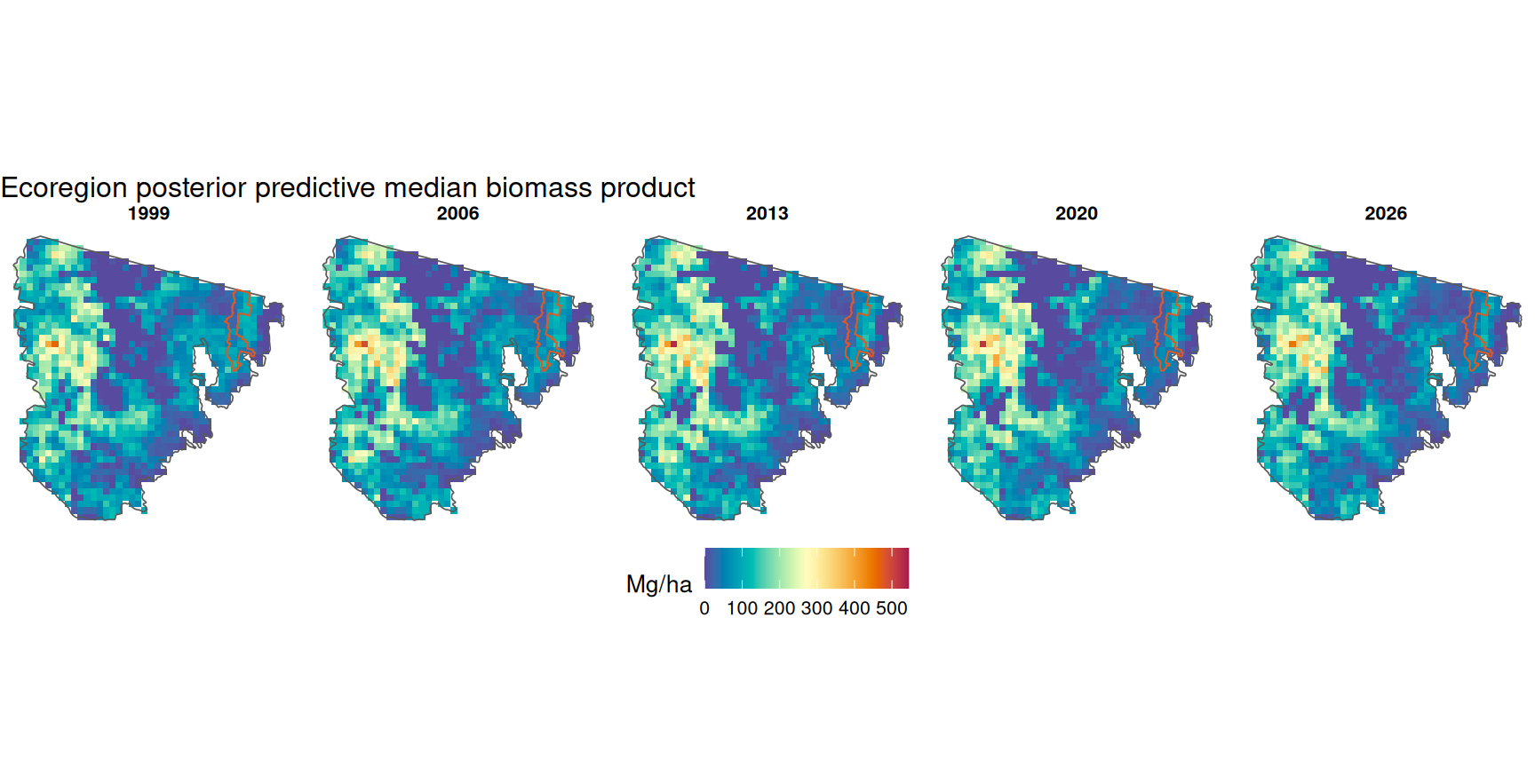
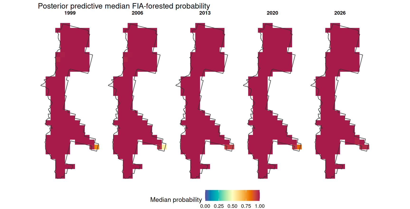
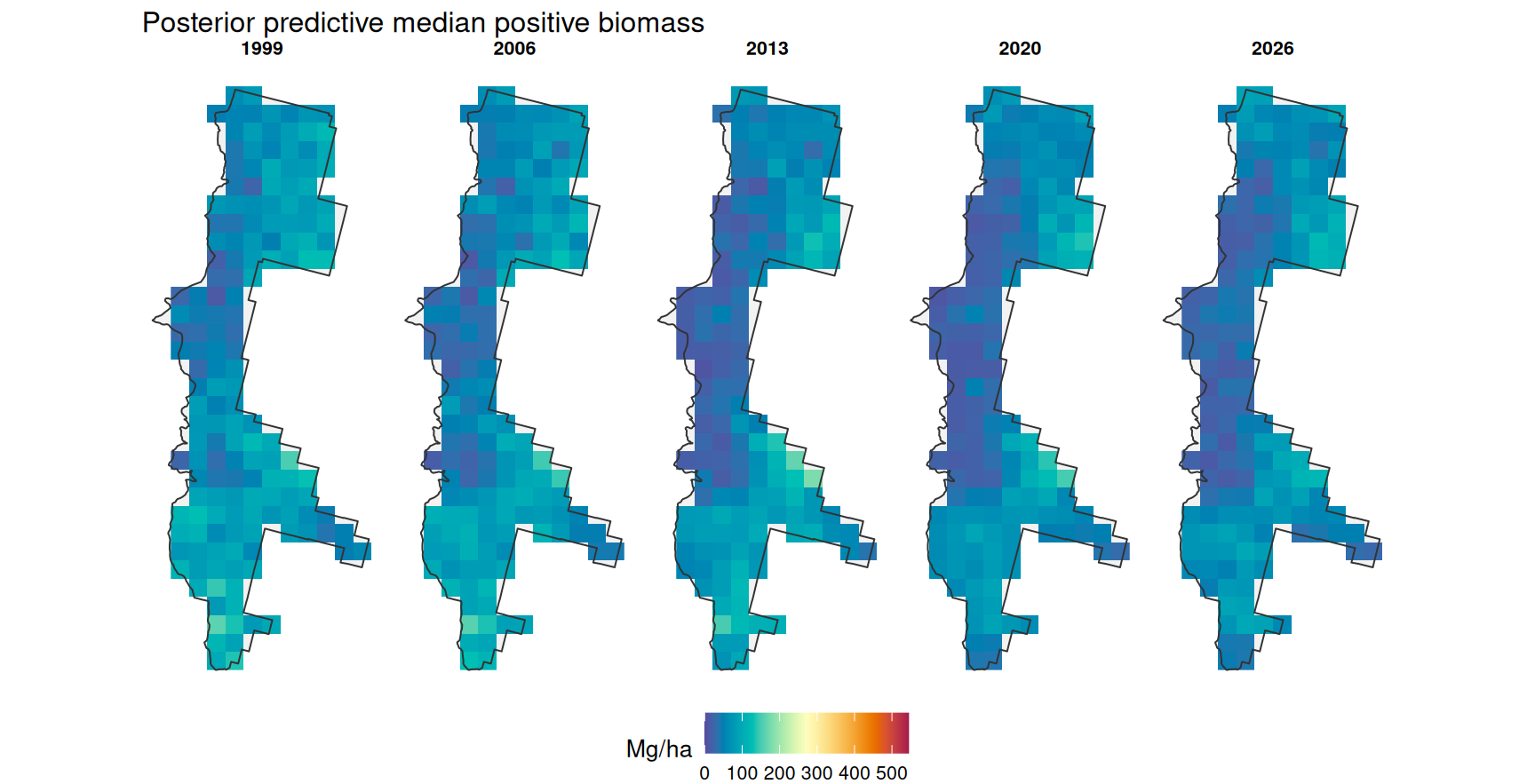
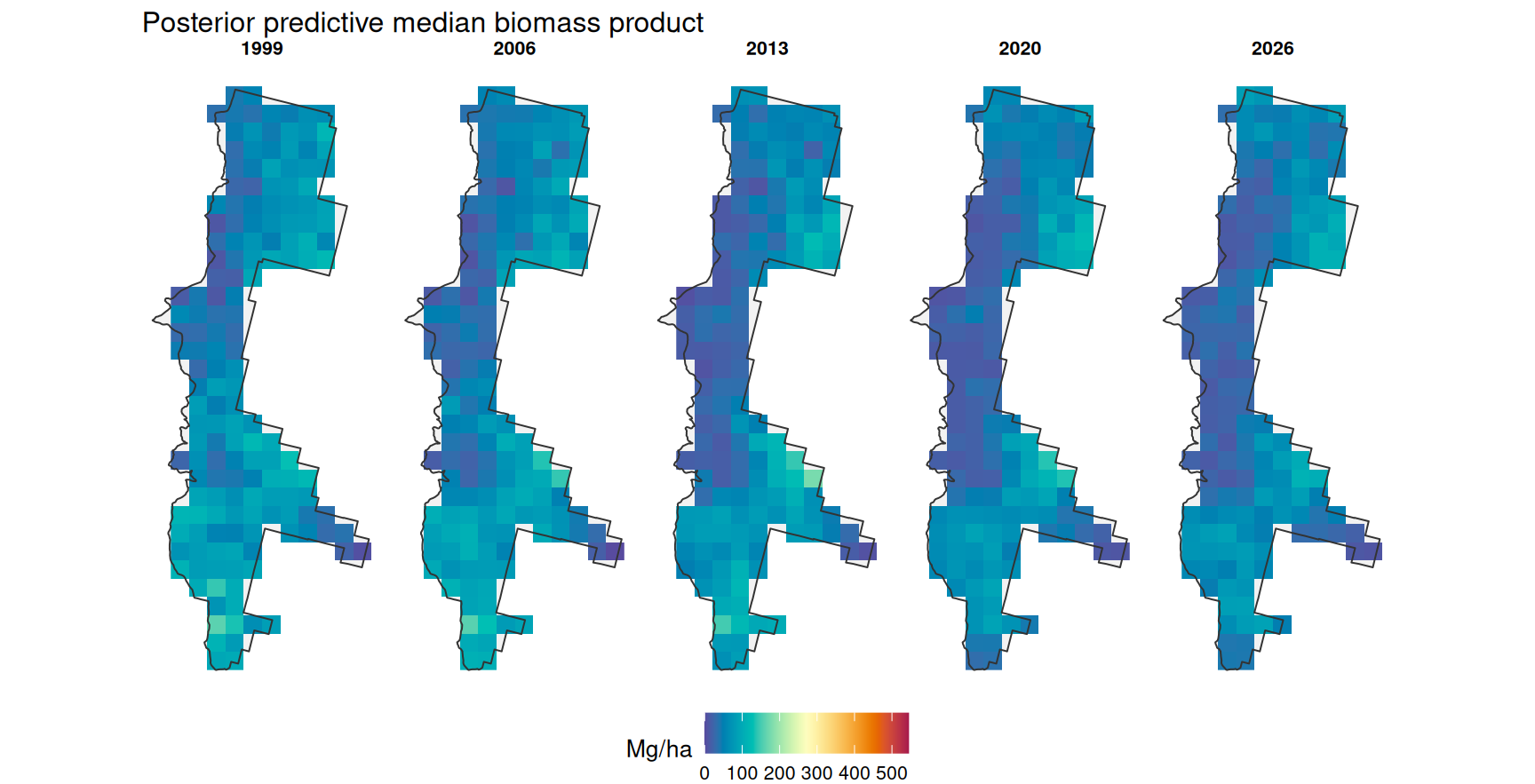
Predictions are made for every year in both grids so the annual summaries can use all years from 1999 through 2026. The maps below show selected years from the joint Vecchia predictions. The ecoregion maps use a 5 km prediction support, and the National Forest maps use a 2 km prediction support. The forest-status map uses posterior median FIA-forested probability. The biomass map uses the posterior predictive median from the Gaussian model after back-transformation to Mg/ha. The product maps use the draw-wise posterior predictive product of FIA-forested status and forested-plot biomass magnitude.

Show summary code
prediction_map_eco_years <- prediction_map_eco %>%
  filter(year %in% map_years)

prediction_map_nf_years <- prediction_map_nf %>%
  filter(year %in% map_years)

biomass_map_limits <- range(
  c(prediction_map_eco$biomass_ppd_median,
    prediction_map_nf$biomass_positive_median,
    prediction_map_nf$biomass_ppd_median)
)

map_theme <- theme_void(base_size = 10) +
  theme(
    legend.position = "bottom",
    strip.text = element_text(face = "bold"),
    plot.title.position = "plot"
  )
Show plotting code
ggplot() +
  geom_sf(data = eco, fill = "grey95", color = NA) +
  geom_raster(data = prediction_map_eco_years,
              aes(x = x, y = y, fill = biomass_ppd_median)) +
  geom_sf(data = eco, fill = NA, color = "grey35", linewidth = 0.3) +
  geom_sf(data = nf, fill = NA, color = stlmm_color("secondary"), linewidth = 0.35) +
  facet_wrap(vars(year), nrow = 1) +
  scale_fill_gradientn(
    colors = stlmm_palette(),
    name = "Mg/ha",
    limits = biomass_map_limits
  ) +
  coord_sf(datum = NA) +
  labs(title = "Ecoregion posterior predictive median biomass product") +
  map_theme

Show plotting code
ggplot() +
  geom_sf(data = nf, fill = "grey95", color = NA) +
  geom_raster(data = prediction_map_nf_years,
              aes(x = x, y = y, fill = forest_prob_median)) +
  geom_sf(data = nf, fill = NA, color = "grey20", linewidth = 0.35) +
  facet_wrap(vars(year), nrow = 1) +
  scale_fill_gradientn(
    colors = stlmm_palette(),
    name = "Median probability",
    limits = c(0, 1)
  ) +
  coord_sf(datum = NA) +
  labs(title = "Posterior predictive median FIA-forested probability") +
  map_theme

Show plotting code
ggplot() +
  geom_sf(data = nf, fill = "grey95", color = NA) +
  geom_raster(data = prediction_map_nf_years,
              aes(x = x, y = y, fill = biomass_positive_median)) +
  geom_sf(data = nf, fill = NA, color = "grey20", linewidth = 0.35) +
  facet_wrap(vars(year), nrow = 1) +
  scale_fill_gradientn(
    colors = stlmm_palette(),
    name = "Mg/ha",
    limits = biomass_map_limits
  ) +
  coord_sf(datum = NA) +
  labs(title = "Posterior predictive median positive biomass") +
  map_theme

Show plotting code
ggplot() +
  geom_sf(data = nf, fill = "grey95", color = NA) +
  geom_raster(data = prediction_map_nf_years,
              aes(x = x, y = y, fill = biomass_ppd_median)) +
  geom_sf(data = nf, fill = NA, color = "grey20", linewidth = 0.35) +
  facet_wrap(vars(year), nrow = 1) +
  scale_fill_gradientn(
    colors = stlmm_palette(),
    name = "Mg/ha",
    limits = biomass_map_limits
  ) +
  coord_sf(datum = NA) +
  labs(title = "Posterior predictive median biomass product") +
  map_theme

9 Annual biomass summaries

Each posterior predictive draw is averaged over a prediction grid within year. The ecoregion summary gives broad context. The National Forest summary approximates the area-average live aboveground biomass density for the Colville National Forest portion in the Northern Cascades. The figure below shows the joint Vecchia summaries for both supports and adds the independent NNGP summary only for the National Forest, where it reproduces the narrower Figure 7-style uncertainty bands from May and Finley (2025).

Show summary code
annual_summary <- function(biomass_ppd_draws, pred_dat, support, prediction_method) {
  grid_year <- pred_dat$year

  annual_draws <- sapply(sort(unique(grid_year)), function(yy) {
    rowMeans(biomass_ppd_draws[, grid_year == yy, drop = FALSE])
  })

  as_tibble(t(apply(
    annual_draws,
    2,
    quantile,
    probs = c(0.025, 0.5, 0.975)
  ))) %>%
    set_names(c("q025", "median", "q975")) %>%
    mutate(year = sort(unique(grid_year)),
           support = support,
           prediction_method = prediction_method) %>%
    relocate(support, prediction_method, year)
}

annual_summary_eco <- annual_summary(eco_product$biomass_ppd_draws,
                                     pred_eco_dat,
                                     "Northern Cascades ecoregion",
                                     "Joint Vecchia")

annual_summary_nf <- annual_summary(nf_product$biomass_ppd_draws,
                                    pred_nf_dat,
                                    "Colville National Forest",
                                    "Joint Vecchia")

annual_summary_nf_independent <- annual_summary(
  nf_product_independent$biomass_ppd_draws,
  pred_nf_dat,
  "Colville National Forest",
  "Independent NNGP"
)

annual_summaries <- bind_rows(annual_summary_eco,
                              annual_summary_nf,
                              annual_summary_nf_independent)

annual_summaries
# A tibble: 84 × 6
   support                     prediction_method  year  q025 median  q975
   <chr>                       <chr>             <int> <dbl>  <dbl> <dbl>
 1 Northern Cascades ecoregion Joint Vecchia      1999  112.   120.  130.
 2 Northern Cascades ecoregion Joint Vecchia      2000  111.   121.  131.
 3 Northern Cascades ecoregion Joint Vecchia      2001  113.   120.  130.
 4 Northern Cascades ecoregion Joint Vecchia      2002  112.   121.  131.
 5 Northern Cascades ecoregion Joint Vecchia      2003  112.   121.  131.
 6 Northern Cascades ecoregion Joint Vecchia      2004  115.   121.  129.
 7 Northern Cascades ecoregion Joint Vecchia      2005  112.   121.  129.
 8 Northern Cascades ecoregion Joint Vecchia      2006  113.   121.  128.
 9 Northern Cascades ecoregion Joint Vecchia      2007  114.   121.  127.
10 Northern Cascades ecoregion Joint Vecchia      2008  114.   121.  128.
# ℹ 74 more rows
Show plotting code
support_levels <- c("Northern Cascades ecoregion", "Colville National Forest")

data_support_lines <- tibble(
  year = c(data_support_start, data_support_dense_end),
  label = c("first FIA measurements", "dense FIA support ends")
)

data_support_labels <- data_support_lines %>%
  mutate(support = factor("Northern Cascades ecoregion",
                          levels = support_levels))

annual_summaries_plot <- annual_summaries %>%
  mutate(
    support = factor(support, levels = support_levels),
    prediction_method = factor(
      prediction_method,
      levels = c("Joint Vecchia", "Independent NNGP")
    )
  )

prediction_method_colors <- c(
  "Joint Vecchia" = stlmm_color("primary"),
  "Independent NNGP" = stlmm_color("contrast")
)

ggplot(annual_summaries_plot, aes(x = year)) +
  geom_vline(
    data = data_support_lines,
    aes(xintercept = year),
    inherit.aes = FALSE,
    linetype = "dashed",
    color = "grey35",
    linewidth = 0.4
  ) +
  geom_ribbon(aes(ymin = q025, ymax = q975, fill = prediction_method),
              alpha = 0.25,
              color = NA) +
  geom_line(aes(y = median,
                color = prediction_method,
                linetype = prediction_method),
            linewidth = 0.9) +
  geom_point(aes(y = median, color = prediction_method), size = 1.5) +
  geom_text(
    data = data_support_labels,
    aes(x = year, y = Inf, label = label),
    inherit.aes = FALSE,
    angle = 90,
    hjust = 1.45,
    vjust = -0.35,
    size = 3,
    color = "grey25"
  ) +
  scale_color_manual(values = prediction_method_colors) +
  scale_fill_manual(values = prediction_method_colors) +
  scale_linetype_manual(values = c("Joint Vecchia" = "solid",
                                   "Independent NNGP" = "dashed")) +
  scale_x_continuous(breaks = seq(1999, 2026, by = 3)) +
  facet_wrap(vars(support), ncol = 1) +
  coord_cartesian(clip = "off") +
  labs(
    x = "Year",
    y = "Live aboveground biomass density (Mg/ha)",
    title = "Posterior predictive biomass distributions",
    subtitle = "The ecoregion uses joint Vecchia only;\nthe National Forest also shows the independent NNGP approximation",
    color = NULL,
    fill = NULL,
    linetype = NULL
  )

10 Summary

This article reproduced the main modeling workflow of May and Finley (2025) for the Colville National Forest portion of the Northern Cascades ecoregion. We prepared FIA plot data, fit a Bernoulli space-time model for FIA-defined forest status, fit a Gaussian space-time model for live aboveground biomass density on FIA-defined forested plots, and used draw-matched posterior predictive samples to form the forested-by-biomass product. We then predicted on annual grids for both the ecoregion and National Forest, mapped selected years, summarized annual biomass distributions, and reviewed fitted spatial-temporal ranges and biomass process-to-noise ratios.

This implementation is intentionally close to, but not identical to, the analysis in May and Finley (2025). One definitional difference is that this article uses FIA forest-condition status for \(z(\mathbf{s}, t)\), whereas the paper defines the binary process from whether biomass is positive. This choice makes the estimates consistent with FIA’s forested definition and with the way the forested-plot biomass model is fit here. The stLMM version also uses the multi_res_sep_exp covariance with a single process variance and an alpha weight to split broad and local components, rather than two separately scaled process variances. The spatial range bounds are chosen to keep the local and landscape components ordered while matching the paper’s scale separation, and the biomass model uses a square-root transformation for a simple nonnegative back-transformation. The NNGP neighbor settings are also lighter than the paper’s full analysis. Finally, the prediction code reports both joint Vecchia prediction and the independent NNGP prediction approximation used for the paper’s Figure 7. These choices provide a compact article implementation while making the main modeling and prediction differences explicit.

In the data preparation, tree biomass from forested conditions was expanded to a per-hectare basis and summed to represent plot-level biomass density. The first-stage response was 1 if the plot had at least one forested condition. Because each plot contributes one 0/1 outcome, this is a Bernoulli observation model, equivalently a binomial model with one trial. That definition is practical, but it discards condition-proportion information. A closer match to FIA’s condition structure would model the forested area proportion directly, for example with a fractional-response or compositional model and is likely a good avenue to explore.

May, Paul B., and Andrew O. Finley. 2025. “Spatial-Temporal Prediction of Forest Attributes Using Latent Gaussian Models and Inventory Data.” Spatial Statistics 69: 100917. https://doi.org/10.1016/j.spasta.2025.100917.