Getting started with stLMM • stLMM

Show preliminaries

library(stLMM)
library(ggplot2)

source(file.path(dirname(knitr::current_input(dir = TRUE)), "utils.R"))

set.seed(1)

1 Overview

This vignette introduces the basic stLMM workflow using small simulated Gaussian response examples. The first model has fixed effects only. The second adds independent and identically distributed (iid) grouped random effects.

The package ships with only a small set of fast vignettes so package checks remain lightweight. Additional model examples, applied workflows, computing notes, and the modeling and software details reference are available on the package website at https://finleya.github.io/stLMM/. The development repository is https://github.com/finleya/stLMM.

2 Fixed-effect model

We start with a simple Gaussian linear model,

\[ y_i = \beta_0 + x_i\beta_1 + \epsilon_i,\qquad \epsilon_i \sim N(0,\tau^2). \]

Code

n <- 50
dat <- data.frame(x = seq(-1, 1, length.out = n))

beta <- c(0.5, -0.5)
tau_sq <- 0.2^2

mu <- beta[1] + beta[2] * dat$x
epsilon <- rnorm(n, sd = sqrt(tau_sq))
dat$y <- mu + epsilon

Show plotting code

ggplot(dat, aes(x, y)) +
  geom_point(
    color = stlmm_color("primary"),
    size = 2
  ) +
  labs(x = "x", y = "response")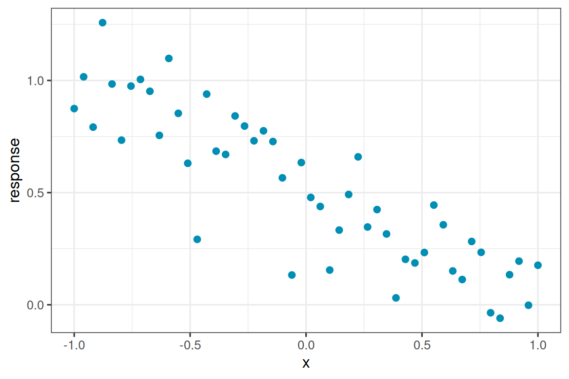

Prior definitions in stLMM state both the parameter they’re associated with and the scale on which the prior distribution is defined. Here the model parameter is the residual variance tau_sq, but half_t(df = 3, scale = 0.5) defines a weakly informative half-\(t\) prior on the residual standard deviation, sqrt(tau_sq), and then transforms that prior internally to the variance scale. In contrast, ig(shape, scale) is placed directly on the variance. See ?stLMM_priors for the parameterization of each prior constructor.

Code

fit <- stLMM(
  y ~ x,
  data = dat,
  priors = list(resid = list(tau_sq = half_t(df = 3, scale = 0.5))),
  n_samples = 250,
  verbose = FALSE
)

summary(fit)

stLMM summary
  formula: y ~ x
  observations: 50
  posterior draws: 250
  family: gaussian
  fixed effects: 2
  grouped random-effect coefficients: 0
  process terms: 0
  residual variance: global tau_sq

beta:
               mean     sd    q2.5   q50.0   q97.5
(Intercept)  0.5193 0.0273  0.4660  0.5185  0.5732
x           -0.5026 0.0447 -0.5956 -0.5034 -0.4223

tau_sq:
        mean     sd   q2.5  q50.0  q97.5
value 0.0302 0.0068 0.0163 0.0291 0.0462

For models without structured process terms, fitted() can be called directly on the fit object.

Code

mu_hat <- fitted(fit)

head(mu_hat)

[1] 1.0218662 1.0013523 0.9808385 0.9603246 0.9398108 0.9192969

Show plotting code

plot_dat <- data.frame(
  x = dat$x,
  y = dat$y,
  fitted = as.numeric(mu_hat)
)

ggplot(plot_dat, aes(x, y)) +
  geom_point(
    color = stlmm_color("primary"),
    size = 2
  ) +
  geom_line(
    aes(y = fitted),
    color = stlmm_color("secondary"),
    linewidth = 0.8
  ) +
  labs(x = "x", y = "response")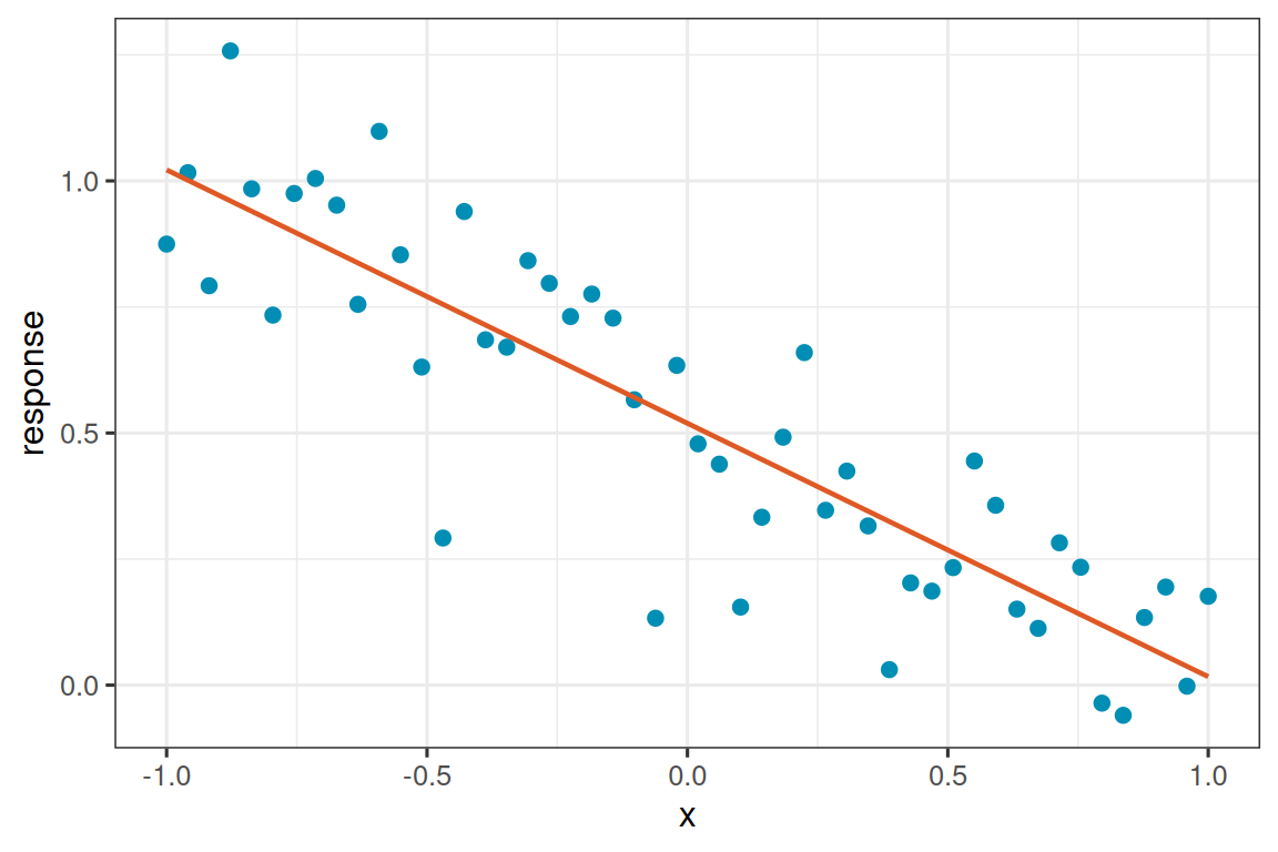

Prediction uses a newdata data frame with the variables needed to rebuild the fixed-effect design matrix.

Code

new_dat <- data.frame(x = c(-0.75, 0, 0.75))

pred <- predict(fit, newdata = new_dat, y_samples = TRUE)

summary(pred)

stLMM prediction summary
  draws: 250
  rows: 3
  newdata: TRUE
  process samples: not retained

mu:
    mean     sd   q2.5  q50.0  q97.5
1 0.8962 0.0447 0.8210 0.8910 0.9877
2 0.5193 0.0273 0.4660 0.5185 0.5732
3 0.1423 0.0417 0.0673 0.1389 0.2294

y:
    mean     sd    q2.5  q50.0  q97.5
1 0.8827 0.1855  0.5249 0.8840 1.2174
2 0.5284 0.1771  0.1494 0.5145 0.8561
3 0.1465 0.1843 -0.1567 0.1426 0.5045

3 Grouped random effects

The iid() term adds exchangeable group-level effects. A random-intercept model is

\[ y_i = \beta_0 + x_i\beta_1 + \alpha_{g_i} + \epsilon_i,\qquad \alpha_g \sim N(0,\sigma_\alpha^2),\quad g=1,\ldots,q. \]

The effects are independent across groups and share a common variance parameter, so iid() is meant literally here: independent and identically distributed group-level effects. Here \(g_i\) is the group level for observation \(i\); in the data, this is the value of the group column for row i.

The residual variance again uses a half-\(t\) prior on the residual standard deviation. In this example, the iid random-effect variance uses an inverse-gamma prior, parameterized by shape and scale.

Code

n_group <- 5
n_per_group <- 10
group_dat <- data.frame(
  group = factor(rep(letters[1:n_group], each = n_per_group)),
  x = rep(seq(-1, 1, length.out = n_per_group), n_group)
)

sigma_sq_alpha <- 0.5^2
alpha_true <- rnorm(n_group, sd = sqrt(sigma_sq_alpha))
names(alpha_true) <- levels(group_dat$group)

beta <- c(0.5, -0.5)
mu <- beta[1] + beta[2] * group_dat$x +
  alpha_true[as.character(group_dat$group)]

tau_sq <- 0.25^2
epsilon <- rnorm(nrow(group_dat), sd = sqrt(tau_sq))
group_dat$y <- mu + epsilon

The call to stLMM() below fits the same model used to generate the data. Parameters associated with model terms are labeled using generated term names. The names combine the term type and an index, where the index gives the order among terms of that same type. For example, this model has one iid() term, so its variance parameter is labeled with iid_1. If the formula had two iid() terms, they would be labeled iid_1 and iid_2 from left to right in the model formula. Structured process terms use the same convention, with names such as nngp_1, car_1, or car_time_1.

Code

group_fit <- stLMM(
  y ~ x + iid(group),
  data = group_dat,
  priors = list(
    resid = list(tau_sq = half_t(df = 3, scale = 0.5)),
    iid_1 = list(sigma_sq = ig(shape = 3, scale = 0.25))
  ),
  n_samples = 250,
  verbose = FALSE
)

summary(group_fit)

stLMM summary
  formula: y ~ x + iid(group)
  observations: 50
  posterior draws: 250
  family: gaussian
  fixed effects: 2
  grouped random-effect coefficients: 5
  process terms: 0
  residual variance: global tau_sq

beta:
               mean     sd    q2.5   q50.0   q97.5
(Intercept)  0.4349 0.2404 -0.1271  0.4244  0.8553
x           -0.5045 0.0563 -0.6098 -0.5057 -0.3944

alpha:
           mean     sd    q2.5   q50.0   q97.5
iid_1_a -0.2324 0.2485 -0.6656 -0.2370  0.2972
iid_1_b  1.4330 0.2513  0.9783  1.4428  1.9955
iid_1_c  0.3719 0.2483 -0.0700  0.3887  0.9236
iid_1_d  0.4871 0.2508  0.0527  0.4874  1.0434
iid_1_e -1.0060 0.2585 -1.4486 -1.0171 -0.4388

tau_sq:
        mean     sd   q2.5  q50.0  q97.5
value 0.0677 0.0132 0.0484 0.0657 0.0947

iid_sigma_sq:
                 mean    sd   q2.5  q50.0  q97.5
iid_1_sigma_sq 0.4514 0.246 0.1974 0.3856 1.0013

Prediction for grouped random effects requires levels that were present during fitting; unseen grouped levels currently produce an error.

Code

group_new <- data.frame(
  group = factor(c("a", "c", "e"), levels = levels(group_dat$group)),
  x = c(-0.5, 0, 0.5)
)

group_pred <- predict(group_fit, newdata = group_new)

summary(group_pred)

stLMM prediction summary
  draws: 250
  rows: 3
  newdata: TRUE
  process samples: not retained

mu:
     mean     sd    q2.5   q50.0   q97.5
1  0.4548 0.0888  0.2926  0.4550  0.6359
2  0.8067 0.0798  0.6539  0.8149  0.9600
3 -0.8234 0.0835 -0.9855 -0.8244 -0.6707

4 Classical SAE model connection

The grouped random-intercept model above connects to a classical unit-level small area estimation (SAE) model. When the response vector holds sampled units and the grouping variable identifies small areas, y ~ x + iid(group) is the model component corresponding to a Bayesian version of the nested-error regression model used by Battese, Harter, and Fuller (BHF) (Battese et al. 1988). In that setting, iid(group) is the area random effect, \(\sigma_\alpha^2\) is the between-area variance, and the Gaussian residual variance is the unit-level error variance.

The classical BHF model uses independent area effects. Spatial or space-time SAE extensions keep the same unit-level response structure but replace iid(group) with structured terms such as car(area, graph = g) or car_time(area, time, graph = g). Area-level estimates are obtained by predicting over the target population support and averaging or summing those predictions.

5 Structured process terms

Structured process terms such as ar1(), gp(), nngp(), car(), and car_time() are handled differently than the iid() term. During fitting, those latent process values are integrated out. After fitting, use recover() to recover the latent random effects for summary or subsequent prediction. That progression looks as follows.

fit <- stLMM(y ~ x + nngp(lon, lat), data = dat, ...)
rec <- recover(fit, sub_sample = list(start = 1001, thin = 5))
fitted(rec)
predict(rec, newdata = new_dat)

Recovered objects can be converted to coda objects just like fitted objects. Use include_w = TRUE when diagnostics or summaries should include recovered latent process draws. For recovered objects, as_mcmc() aligns fixed-effect, variance, covariance, and recovered process columns to the same posterior iterations selected by recover().

rec_mcmc <- as_mcmc(rec, include_w = TRUE)

Later vignettes cover point-referenced, areal, space-time, binomial, residual variance, and sampler-diagnostic workflows.

Battese, George E., Rachel M. Harter, and Wayne A. Fuller. 1988. “An Error-Components Model for Prediction of County Crop Areas Using Survey and Satellite Data.” Journal of the American Statistical Association 83 (401): 28–36. https://doi.org/10.1080/01621459.1988.10478561.