
Spatial NNGP models with stLMM
Point-referenced spatial effects, recovery, and holdout prediction
Source:vignettes/v02-spatial-nngp.qmd
1 Overview
This vignette introduces point-referenced spatial process terms using nngp(). We simulate a Gaussian response from a full spatial Gaussian process with an exponential covariance function, fit the training data with a nearest neighbor Gaussian process (NNGP) approximation, recover the fitted spatial random effects, and predict held-out observations.
2 Model
For observation \(i\) at location \(\mathbf{s}_i = (s_{i1}, s_{i2})^\top\), the model is
\[ y_i = \beta_0 + x_i\beta_1 + w(\mathbf{s}_i) + \epsilon_i,\qquad \epsilon_i \sim N(0,\tau^2). \]
The spatial process is
\[ \mathbf{w} = \{w(\mathbf{s}_1),\ldots,w(\mathbf{s}_n)\}^\top \sim N(\mathbf{0}, \sigma^2 \mathbf{R}(\phi)), \]
where the exponential correlation function is
\[ R_{ij}(\phi) = \exp\{-\phi \|\mathbf{s}_i - \mathbf{s}_j\|\}. \]
The full Gaussian process covariance is used to simulate the data. The fitted model uses nngp(), which approximates the full process with a sparse nearest-neighbor representation. Datta et al. (2016) introduced NNGP models as scalable fully model-based Gaussian process models for large geostatistical datasets. The implementation here uses the same NNGP model idea, but the latent spatial effects are integrated out during fitting. This lets the MCMC target the fixed-effect and covariance parameters directly; fitted-support process values are then drawn afterward with recover(). This workflow follows the sparse Bayesian NNGP algorithms in Finley et al. (2019).
3 Data
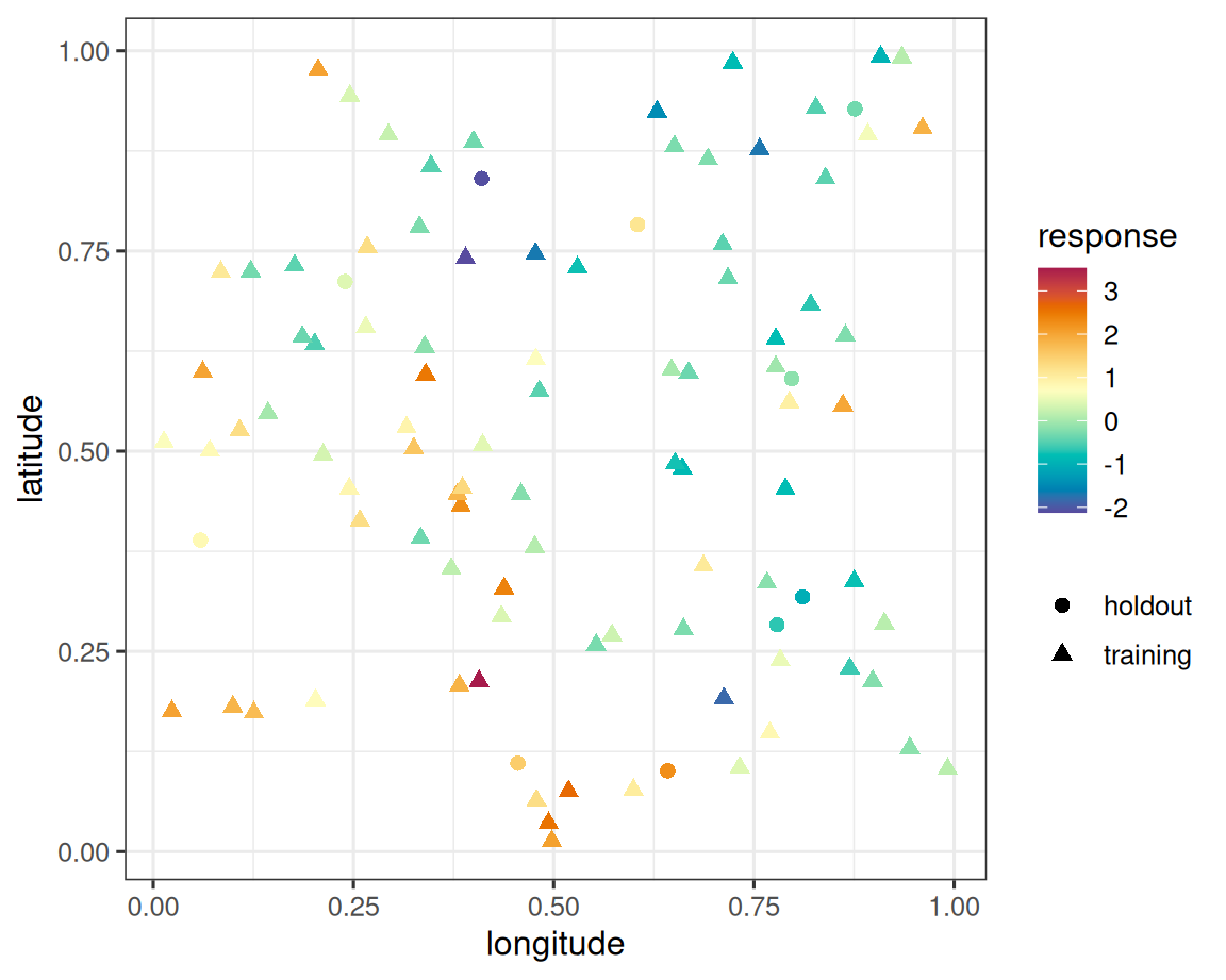
We simulate locations in the unit square, then set aside 10 locations for prediction. The observed response combines a linear mean, a spatial random effect, and independent Gaussian noise.
Code
n_train <- 90
n_holdout <- 10
n <- n_train + n_holdout

dat <- data.frame(
  lon = runif(n),
  lat = runif(n),
  x = runif(n, -1, 1)
)

beta <- c(0.5, 1)
sigma_sq <- 1
phi <- 4
tau_sq <- 0.1

C <- exp_cov(
  coords = dat[, c("lon", "lat")],
  sigma_sq = sigma_sq,
  phi = phi
)

dat$w_true <- rmvnorm(mean = rep(0, n), Sigma = C)

mu <- beta[1] + beta[2] * dat$x + dat$w_true
epsilon <- rnorm(n, sd = sqrt(tau_sq))
dat$y <- mu + epsilon

train <- dat[1:n_train, ]
holdout <- dat[(n_train + 1):n, ]
Show plotting code
plot_dat <- rbind(
  data.frame(train, sample = "training"),
  data.frame(holdout, sample = "holdout")
)

ggplot(plot_dat, aes(lon, lat)) +
  geom_point(
    aes(color = y, shape = sample),
    size = 2.2
  ) +
  scale_color_gradientn(colors = stlmm_palette()) +
  coord_equal() +
  labs(
    x = "longitude",
    y = "latitude",
    color = "response",
    shape = NULL
  )
4 Fit
The simulated data were generated from a full Gaussian process with the exponential covariance model. The fitted model below uses nngp() as a nearest-neighbor approximation to that full Gaussian process. The approximation keeps the same covariance function but replaces dense full Gaussian process calculations with sparse nearest-neighbor calculations.
The formula adds an NNGP spatial process over the coordinate columns lon and lat. The argument m = 15 uses up to 15 previously ordered neighbors for each process node. The ordering = "maxmin" option often gives a useful ordering for spatial NNGP and Vecchia-type approximations; see Guinness (2018) and Katzfuss and Guinness (2021) for discussion of how ordering can affect approximation quality. For large datasets, exact max-min ordering can be slower than coordinate or Hilbert orderings.
The residual and process variances use half-\(t\) priors on their corresponding standard deviations. The spatial decay parameter phi uses a bounded uniform prior. For the exponential correlation model, larger phi means correlation decays more quickly with distance.
Code
stLMM summary
  formula: y ~ x + nngp(lon, lat, m = 15, cov_model = "exp", ordering = "maxmin")
  observations: 90
  posterior draws: 500
  family: gaussian
  fixed effects: 2
  grouped random-effect coefficients: 0
  process terms: 1
  residual variance: global tau_sq

beta:
              mean     sd    q2.5  q50.0  q97.5
(Intercept) 0.7694 0.4909 -0.1674 0.7501 1.8647
x           1.0905 0.1163  0.8685 1.0868 1.3113

tau_sq:
       mean     sd   q2.5  q50.0  q97.5
value 0.084 0.0573 0.0057 0.0728 0.2272

sigma_sq:
                  mean     sd  q2.5  q50.0  q97.5
nngp_1_sigma_sq 1.1467 0.3222 0.644 1.0796 1.8624

theta:
             mean     sd   q2.5  q50.0  q97.5
nngp_1_phi 3.8978 1.2433 2.2759 3.6849 7.2063
5 Recover
Structured process terms are integrated out during fitting. The posterior samples above contain covariance and fixed-effect parameters, but not the latent process values in a directly usable form. Calling recover() draws the fitted spatial random effects conditional on the retained posterior parameter samples.
stLMM recovery
  formula: y ~ x + nngp(lon, lat, m = 15, cov_model = "exp", ordering = "maxmin")
  observations: 90
  recovered draws: 150
  recovered process terms: nngp_1
Use as_mcmc(rec, include_w = TRUE) when you want a coda::mcmc object with parameter samples and recovered process draws on the same posterior iterations. The examples below use as_samples() only because data-frame columns are convenient for ggplot2.
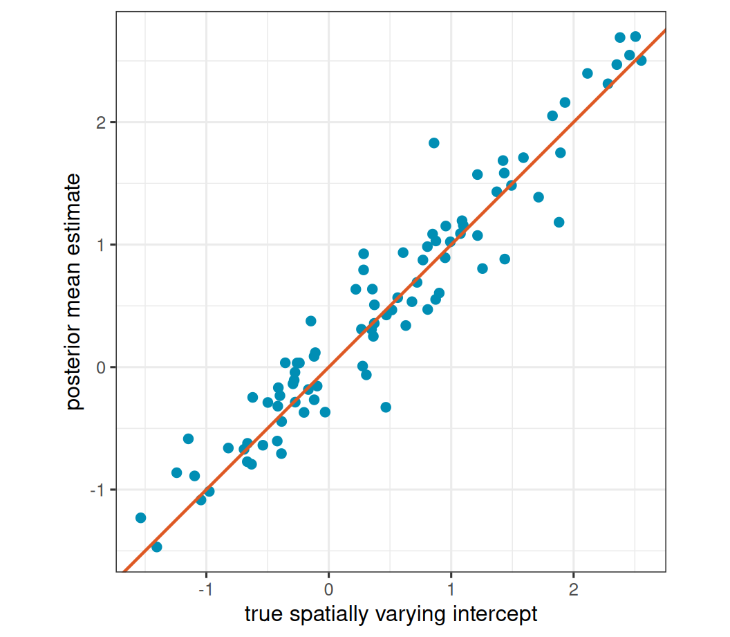
Because this example has one observation at each training location, the recovered nngp_1 columns correspond to the training rows. The data identify the combined spatially varying intercept, \(\beta_0 + w(\mathbf{s}_i)\), more directly than its split into a global intercept and one realized spatial process. For this diagnostic, we compare \(\beta_0 + w(\mathbf{s}_i)\) rather than \(w(\mathbf{s}_i)\) alone.
Show plotting code
rec_draws <- as_samples(rec, include_w = TRUE, metadata = FALSE)
w_cols <- paste0("w_nngp_1_", seq_len(nrow(train)))
w_hat <- colMeans(rec_draws[, w_cols, drop = FALSE])
beta_0_hat <- mean(rec_draws[["(Intercept)"]])

recovery_dat <- data.frame(
  truth = beta[1] + train$w_true,
  estimate = beta_0_hat + w_hat
)

ggplot(recovery_dat, aes(truth, estimate)) +
  geom_point(
    color = stlmm_color("primary"),
    size = 2
  ) +
  geom_abline(
    intercept = 0,
    slope = 1,
    color = stlmm_color("secondary"),
    linewidth = 0.8
  ) +
  coord_equal() +
  labs(
    x = "true spatially varying intercept",
    y = "posterior mean estimate"
  )
6 Predict
Prediction at new locations uses the recovered NNGP process draws. With joint = FALSE, each new prediction location is simulated independently conditional on its nearest fitted-support neighbors. This is usually sufficient when the goal is a marginal posterior mean, interval, or prediction map. Use joint = TRUE when the dependence among prediction locations matters, for example when summaries involve averages, totals, contrasts, exceedance areas, or other functions of multiple predicted locations.
Code
stLMM prediction summary
  draws: 150
  rows: 10
  newdata: TRUE
  process samples: not retained

mu:
       mean     sd    q2.5   q50.0   q97.5
91  -0.2577 0.4695 -1.2330 -0.2452  0.8231
92   0.6178 0.7033 -0.7762  0.6209  1.8740
93   2.1006 0.4998  1.0186  2.1196  2.9453
94   0.0977 0.4302 -0.7210  0.0593  0.8593
95  -0.5681 0.4780 -1.5036 -0.6000  0.5205
96   0.6871 0.3817 -0.0573  0.6673  1.4336
97   1.4235 0.5329  0.2919  1.4530  2.2785
98  -1.9110 0.5211 -2.8914 -1.9122 -0.9204
99  -1.3603 0.4502 -2.1925 -1.3349 -0.4535
100  0.1731 0.5200 -0.7797  0.1472  1.1548

y:
       mean     sd    q2.5   q50.0   q97.5
91  -0.2470 0.5930 -1.4908 -0.1962  0.7087
92   0.6295 0.7435 -0.8087  0.5911  1.9556
93   2.1046 0.5918  0.8581  2.0981  3.2116
94   0.0825 0.5472 -1.0694  0.0653  1.1086
95  -0.5712 0.5675 -1.5420 -0.6174  0.5546
96   0.7064 0.4873 -0.2691  0.6756  1.6432
97   1.4102 0.6247  0.2174  1.4156  2.5015
98  -1.9380 0.5658 -2.8685 -2.0123 -0.8319
99  -1.3625 0.5185 -2.2966 -1.3931 -0.1330
100  0.1687 0.5771 -1.0230  0.1588  1.2892
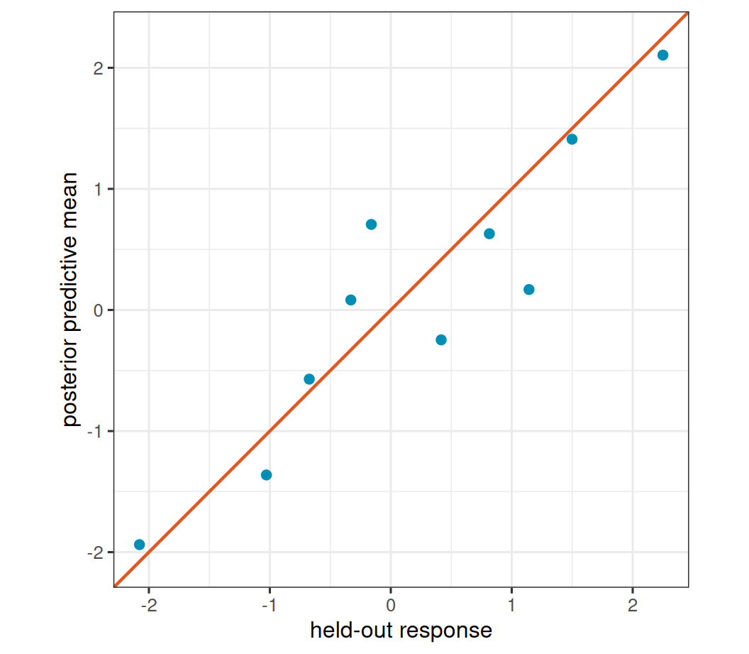
The predict() call returns posterior draws of \(\mu\) and, when y_samples = TRUE, posterior predictive response draws. As shown above, passing the prediction object to summary() gives posterior summaries for these draws. Setting return_w_samples = TRUE also retains the predicted latent process draws for each process term.
Show plotting code
pred_draws <- as_samples(pred, sample = "all", metadata = FALSE)
mu_cols <- paste0("mu_", seq_len(nrow(holdout_new)))
y_cols <- paste0("y_", seq_len(nrow(holdout_new)))
mu_hat <- colMeans(pred_draws[, mu_cols, drop = FALSE])
y_hat <- colMeans(pred_draws[, y_cols, drop = FALSE])

pred_dat <- data.frame(
  y = holdout$y,
  mu_hat = mu_hat,
  y_hat = y_hat
)
pred_lim <- range(pred_dat$y, pred_dat$y_hat)

ggplot(pred_dat, aes(y, y_hat)) +
  geom_point(
    color = stlmm_color("primary"),
    size = 2
  ) +
  geom_abline(
    intercept = 0,
    slope = 1,
    color = stlmm_color("secondary"),
    linewidth = 0.8
  ) +
  coord_equal(
    xlim = pred_lim,
    ylim = pred_lim
  ) +
  labs(
    x = "held-out response",
    y = "posterior predictive mean"
  )
7 What this example illustrates
The main workflow difference from fixed-effect and iid random-effect models is the recovery step. NNGP process values are integrated out during fitting, so recover() is needed before using process contributions in fitted values or prediction.
This example also shows the separation between the covariance model and the approximation. The data were simulated from a full exponential Gaussian process, while nngp() used a nearest-neighbor approximation with the same exponential covariance function. For larger spatial datasets, the NNGP approximation is the scalable option.
8 Full GP comparison
For very small point-referenced datasets, stLMM also provides a dense full Gaussian process term through gp(). The model below swaps nngp() for gp() while leaving the rest of the formula and prior structure unchanged.
Code
stLMM summary
  formula: y ~ x + gp(lon, lat, cov_model = "exp")
  observations: 90
  posterior draws: 500
  family: gaussian
  fixed effects: 2
  grouped random-effect coefficients: 0
  process terms: 1
  residual variance: global tau_sq

beta:
              mean     sd    q2.5  q50.0  q97.5
(Intercept) 0.7688 0.5150 -0.1708 0.7799 1.8785
x           1.0862 0.1135  0.8683 1.0855 1.3080

tau_sq:
        mean    sd   q2.5  q50.0 q97.5
value 0.0871 0.053 0.0082 0.0796 0.202

sigma_sq:
                mean     sd   q2.5  q50.0  q97.5
gp_1_sigma_sq 1.2299 0.4021 0.6937 1.1349 2.1912

theta:
           mean     sd   q2.5  q50.0  q97.5
gp_1_phi 3.6442 1.1555 2.1038 3.5289 6.1342
The dense gp() term is included mainly as a small-data reference and testing tool. The package emphasis is on models that use sparse precision matrices or sparse approximations, such as nngp(), ar1(), car(), and car_time(). Dense GP covariance calculations scale poorly as the number of unique locations grows, so gp() should not be treated as the default spatial workflow for large datasets.