
Direct-estimate CAR-time model with TCC
Area-response smoothing with a remote-sensing covariate
Source:vignettes/wa-direct-car-time-scaled-variance-tcc.qmd
1 Purpose
This article extends the scaled-variance direct-estimate CAR-time model by adding county mean tree canopy cover (TCC) as an auxiliary predictor. The response is a county-year direct estimate of live aboveground biomass density, and the inferential target remains the latent county-year biomass mean.
This is an area-response model: each row represents a county-year, not a plot. It follows the Fay-Herriot small-area model structure (Fay and Herriot 1979), with a CAR-time process replacing an independent area effect. The TCC covariate enters the latent mean model, while the supplied direct-estimate variances remain a variance template that the model can recalibrate.
Source code and data links for reproducing this article are collected below.
2 Model
Let \(i\) index an observed county-year direct estimate, with county \(a_i\) and year \(t_i\). The direct estimate \(\hat{y}_i\) is modeled as
\[ \hat{y}_i = \theta_i + e_i,\qquad e_i \sim N(0,\tau_i^2), \]
where \(\theta_i = \theta_{a_i,t_i}\) is the latent county-year biomass mean and \(\tau_i^2\) is the observation variance for the direct estimate. The latent mean model is
\[ \theta_i = \beta_0 + \beta_1 x_i + w_{a_i,t_i}, \]
where \(x_i\) is standardized county mean TCC and \(w_{a,t}\) is a separable CAR-time process over counties and years. Its spatial component is defined by the county graph, and its temporal component is defined over the annual support.
The supplied direct-estimate variance \(\hat{v}_i\) enters through a scaled residual variance model. With effective sample size \(n_i\) and fixed shrinkage constant \(c = 10\), the observation variance is
\[ \log(\tau_i^2) = \log(\kappa) + \omega_i\log(\hat{v}_i) + (1 - \omega_i)\log(\tau_0^2), \qquad \omega_i = \frac{n_i}{n_i + c}. \]
The positive scaling parameter \(\kappa\) lets the model learn whether the supplied direct-estimate variances are too small or too large overall. The common scale \(\tau_0^2\) gives low-sample-size direct estimates a place to shrink toward on the log-variance scale.
Some multi-plot county-years have zero raw direct-estimate variance because all sampled plots have zero biomass. Those rows contain useful information, but a zero observation variance would treat the direct estimate as exact. The data bundle therefore assigns them a small positive floor, equal to the 5th percentile of the positive raw direct-estimate variances. In this article the floor is only a variance template: the scaled residual variance model recalibrates it using \(\kappa\), \(\tau_0^2\), and \(n_i\).
3 Data
The data chunk below reads the county polygons and county-year direct estimates. Rows with missing direct_biomass_model are retained because they define county-year latent support for recovery and fitted values, but they do not contribute to the likelihood.
Show data-reading code
wa_counties <- read_rds(file.path(data_dir, "wa_counties.rds"))
direct_estimates <- read_csv(file.path(data_dir, "wa_direct_estimates.csv"), show_col_types = FALSE)

wa_counties <- wa_counties |>
  mutate(county_fips = as.character(county_fips))

direct_estimates <- direct_estimates |>
  mutate(
    county_fips = as.character(county_fips),
    year = as.integer(year),
    county_mean_tcc_scaled = as.numeric(scale(county_mean_tcc))
  ) |>
  arrange(county_fips, year)

observed_direct <- direct_estimates |>
  filter(!is.na(direct_biomass_model))
The table summarizes the area-response data used in this article. County-years with a single FIA plot remain in the county-year support, but they are not used as direct-estimate likelihood rows because their design-based variance cannot be estimated from one plot.
Show data summary code
direct_summary <- tibble(
  quantity = c(
    "counties",
    "years",
    "county-years",
    "model-ready direct estimates",
    "missing model responses",
    "single-plot rows retained but excluded",
    "variance-floor rows",
    "median plot count among modeled county-years",
    "median direct-estimate SE"
  ),
  value = c(
    n_distinct(direct_estimates$county_fips),
    n_distinct(direct_estimates$year),
    nrow(direct_estimates),
    sum(direct_estimates$direct_estimate_in_model),
    sum(is.na(direct_estimates$direct_biomass_model)),
    sum(direct_estimates$direct_estimate_status == "single_plot_no_variance"),
    sum(direct_estimates$direct_estimate_in_model &
          direct_estimates$direct_biomass_vhat_source == "floor", na.rm = TRUE),
    median(observed_direct$n, na.rm = TRUE),
    median(observed_direct$direct_biomass_se_model, na.rm = TRUE)
  )
) |>
  mutate(value = fmt_num(as.numeric(value), 1))

show_table(direct_summary, caption = "County-year direct-estimate data used in the scaled-variance CAR-time model.")| quantity | value |
|---|---|
| counties | 39.0 |
| years | 10.0 |
| county-years | 390.0 |
| model-ready direct estimates | 315.0 |
| missing model responses | 75.0 |
| single-plot rows retained but excluded | 15.0 |
| variance-floor rows | 60.0 |
| median plot count among modeled county-years | 19.0 |
| median direct-estimate SE | 23.6 |
The next table shows selected-year data coverage. The model includes all counties in every year, but years with fewer observed direct estimates rely more heavily on the model structure.
Show year coverage code
year_coverage <- direct_estimates |>
  group_by(year) |>
  summarise(
    counties_with_direct_estimates = sum(direct_estimate_in_model),
    median_plot_n = median(n[n > 0], na.rm = TRUE),
    median_direct_biomass = median(direct_biomass_model, na.rm = TRUE),
    median_direct_se = median(direct_biomass_se_model, na.rm = TRUE),
    .groups = "drop"
  )

show_table(
  year_coverage |>
    filter(year %in% c(2016, 2018, 2020, 2022, 2024, 2025)) |>
    mutate(
      median_plot_n = fmt_num(median_plot_n, 0),
      median_direct_biomass = fmt_num(median_direct_biomass, 1),
      median_direct_se = fmt_num(median_direct_se, 1)
    ),
  caption = "Selected-year direct-estimate coverage and precision."
)| year | counties_with_direct_estimates | median_plot_n | median_direct_biomass | median_direct_se |
|---|---|---|---|---|
| 2016 | 39 | 22 | 90.3 | 23.6 |
| 2018 | 38 | 22 | 84.1 | 22.2 |
| 2020 | 36 | 18 | 51.8 | 17.9 |
| 2022 | 37 | 21 | 72.7 | 12.9 |
| 2024 | 18 | 3 | 136.3 | 75.4 |
| 2025 | 0 | NA | NA | NA |
4 County Mean TCC
County mean TCC is computed from the annual USDA Forest Service Tree Canopy Cover raster products for each county-year (USDA Forest Service 2026). The model uses a standardized version of this covariate so the fixed-effect coefficient is measured per one standard deviation increase in county mean TCC.
Show TCC summary code
tcc_summary <- direct_estimates |>
  summarise(
    mean_tcc = mean(county_mean_tcc, na.rm = TRUE),
    sd_tcc = sd(county_mean_tcc, na.rm = TRUE),
    min_tcc = min(county_mean_tcc, na.rm = TRUE),
    max_tcc = max(county_mean_tcc, na.rm = TRUE),
    observed_cor = cor(direct_biomass_model, county_mean_tcc, use = "complete.obs")
  ) |>
  pivot_longer(everything(), names_to = "quantity", values_to = "value") |>
  mutate(
    quantity = recode(
      quantity,
      mean_tcc = "mean county TCC",
      sd_tcc = "SD county TCC",
      min_tcc = "minimum county TCC",
      max_tcc = "maximum county TCC",
      observed_cor = "correlation with direct biomass"
    ),
    value = fmt_num(value, 2)
  )

show_table(tcc_summary, caption = "County-year TCC summary.")| quantity | value |
|---|---|
| mean county TCC | 38.15 |
| SD county TCC | 23.71 |
| minimum county TCC | 1.84 |
| maximum county TCC | 70.75 |
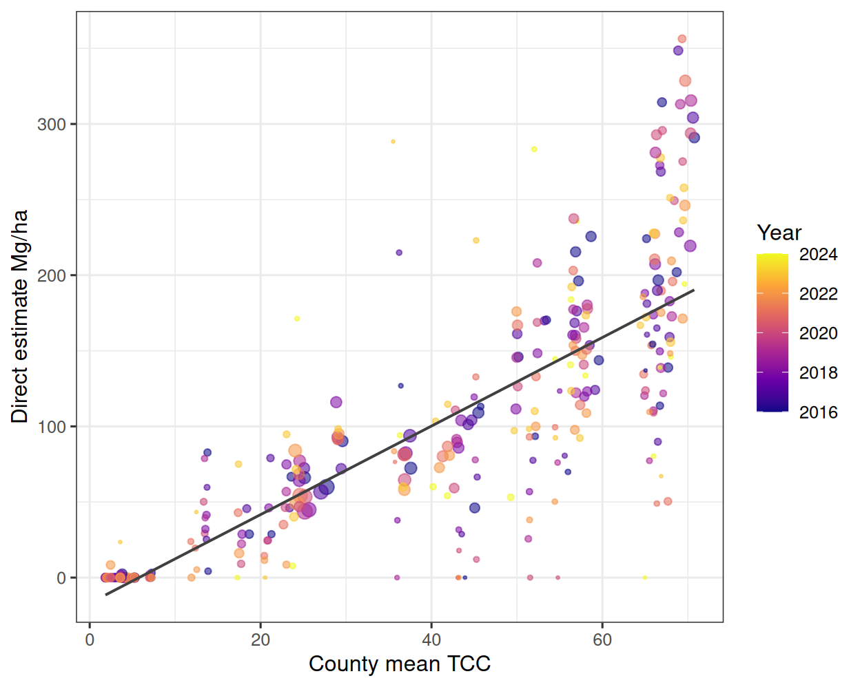
| correlation with direct biomass | 0.80 |
The scatter plot shows the observed relationship between county mean TCC and direct-estimate biomass. The model does not use this relationship alone; it estimates the TCC effect jointly with the CAR-time process and the scaled observation variances.
Show TCC direct-estimate scatter code
ggplot(observed_direct, aes(x = county_mean_tcc, y = direct_biomass_model)) +
  geom_point(aes(size = n_eff_model, color = year), alpha = 0.55) +
  geom_smooth(method = "lm", se = FALSE, color = "grey25", linewidth = 0.7) +
  scale_size_continuous(range = c(0.5, 3.5), guide = "none") +
  scale_color_viridis_c(option = "C") +
  labs(
    x = "County mean TCC",
    y = "Direct estimate Mg/ha",
    color = "Year"
  )
5 County Graph
The county graph defines spatial neighbors for the CAR component. Washington has island components, so the graph construction explicitly adds nearest-neighbor bridge edges. The island rule is part of the model definition.
g <- car_graph(
  wa_counties,
  id = "county_fips",
  island = "nearest",
  island_k = 4
)

g$island_added_edges
from to distance
1 53055 53029 56295.37
2 53055 53035 100453.91
3 53055 53073 100817.65
4 53055 53057 102288.11The figure checks the graph visually. Thin lines connect neighboring county centroids; thicker colored lines show bridge edges added for island components.
Show graph plotting code
coord_dat <- data.frame(
  county_fips = wa_counties$county_fips,
  sf::st_coordinates(sf::st_point_on_surface(sf::st_geometry(wa_counties)))
)

edge_index <- which(as.matrix(g$adjacency) != 0, arr.ind = TRUE)
edge_index <- edge_index[edge_index[, "row"] < edge_index[, "col"], , drop = FALSE]
edge_dat <- tibble(
  from = g$ids[edge_index[, "row"]],
  to = g$ids[edge_index[, "col"]]
) |>
  mutate(
    key = paste(pmin(from, to), pmax(from, to), sep = "--"),
    x = coord_dat$X[match(from, coord_dat$county_fips)],
    y = coord_dat$Y[match(from, coord_dat$county_fips)],
    xend = coord_dat$X[match(to, coord_dat$county_fips)],
    yend = coord_dat$Y[match(to, coord_dat$county_fips)]
  )

island_key <- paste(
  pmin(g$island_added_edges$from, g$island_added_edges$to),
  pmax(g$island_added_edges$from, g$island_added_edges$to),
  sep = "--"
)
edge_dat$island <- edge_dat$key %in% island_key

ggplot(wa_counties) +
  geom_sf(fill = "grey96", color = "white", linewidth = 0.15) +
  geom_segment(
    data = edge_dat,
    aes(x = x, y = y, xend = xend, yend = yend, color = island, linewidth = island)
  ) +
  geom_point(data = coord_dat, aes(X, Y), color = stlmm_color("primary"), size = 1.3) +
  coord_sf(expand = FALSE) +
  scale_color_manual(
    values = c("FALSE" = "grey45", "TRUE" = stlmm_color("secondary")),
    guide = "none"
  ) +
  scale_linewidth_manual(values = c("FALSE" = 0.25, "TRUE" = 1), guide = "none")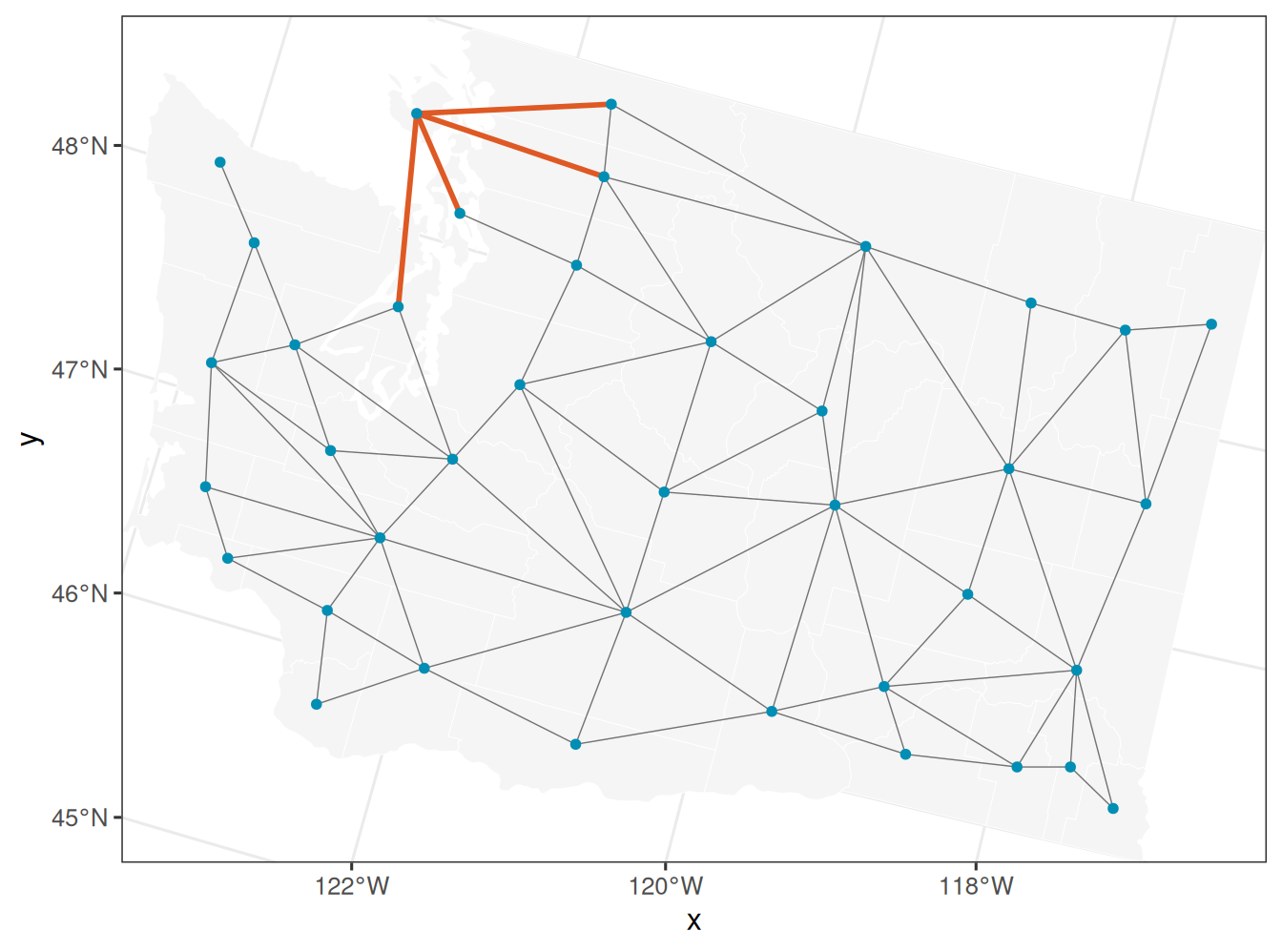
6 Fit
The sampler settings below are chosen to give stable posterior summaries for the example while keeping the workflow practical to rerun. For a final analysis, increase the run length as needed and check convergence diagnostics before interpreting results.
n_samples <- 12000
burnin <- 6000
chains <- 3
n_keep <- 100
posterior_thin <- max(1L, floor((n_samples - burnin) / n_keep))
posterior_sub_sample <- list(start = burnin + 1, thin = posterior_thin)
chain_control <- list(seed = 1, dispersion = 1.5)
warmup_control <- list(batch_length = 25, min_batches = 10)
summary_parameters <- c(
  "(Intercept)",
  "county_mean_tcc_scaled",
  "kappa",
  "tau0_sq",
  "car_time_1_sigma_sq",
  "car_time_1_rho",
  "car_time_1_phi"
)
The n_keep value controls how many post-burn-in draws per chain are retained for recovery and fitted-value summaries. The fit summary uses all post-burn-in MCMC samples.
In the model call below, direct_biomass_model is \(\hat{y}_i\), county_mean_tcc_scaled is \(x_i\), direct_biomass_vhat_model is \(\hat{v}_i\), and n_eff_model is \(n_i\). Scaled direct-estimate variances enter through resid(model = "scaled", variance = direct_biomass_vhat_model, n = n_eff_model).
fit <- stLMM(
  direct_biomass_model ~
    county_mean_tcc_scaled +
    car_time(county_fips, year, graph = g, car_model = "leroux") +
    resid(
      model = "scaled",
      variance = direct_biomass_vhat_model,
      n = n_eff_model,
      shrinkage = 10,
      kappa_log_prior = c(mean = 0, sd = 1)
    ),
  data = direct_estimates,
  priors = list(
    car_time_1 = list(
      sigma_sq = half_t(
        df = 3,
        scale = sd(observed_direct$direct_biomass_model, na.rm = TRUE)
      ),
      rho = uniform(0.01, 0.99),
      phi = uniform(-0.99, 0.99)
    )
  ),
  n_samples = n_samples,
  chains = chains,
  chain_control = chain_control,
  warmup = warmup_control,
  verbose = TRUE,
  n_report = 500
)

fit_summary <- summary(fit, burn = burnin, parameters = summary_parameters)
Show fit summary code
fit_summarystLMM multi-chain summary
formula: direct_biomass_model ~ county_mean_tcc_scaled + car_time(county_fips, year, graph = g, car_model = "leroux") + resid(model = "scaled", variance = direct_biomass_vhat_model, n = n_eff_model, shrinkage = 10, kappa_log_prior = c(mean = 0, sd = 1))
chains: 3
family: gaussian
observations: 390 (315 observed, 75 missing response)
posterior draws per chain: 12000 (6000 used after burn = 6000)
process terms: 1
Parameters:
mean sd q2.5 q50.0 q97.5
(Intercept) 88.6364 11.1357 66.2062 88.7793 110.6086
county_mean_tcc_scaled 73.2892 7.4813 59.3491 73.0456 88.5773
kappa 0.5959 0.1123 0.4104 0.5826 0.8399
tau0_sq 7650.6436 3099.9144 3321.1841 7069.9048 15276.7134
car_time_1_sigma_sq 2136.3419 681.2171 1050.9640 2067.8879 3665.6174
car_time_1_rho 0.4200 0.2015 0.0722 0.4106 0.8154
car_time_1_phi 0.9867 0.0037 0.9767 0.9880 0.9899
Chain diagnostics:
parameter rhat effective_size
(Intercept) (Intercept) 1.0006 18419.5539
county_mean_tcc_scaled county_mean_tcc_scaled 1.0001 5256.7400
kappa kappa 1.0030 1092.0759
tau0_sq tau0_sq 1.0046 1127.5745
car_time_1_sigma_sq car_time_1_sigma_sq 1.0010 831.8046
car_time_1_rho car_time_1_rho 1.0018 798.4272
car_time_1_phi car_time_1_phi 1.0010 1284.4580The county_mean_tcc_scaled row estimates the mean-model association between county mean TCC and latent county-year biomass after accounting for CAR-time structure and direct-estimate uncertainty. Because the covariate is standardized, the coefficient is the expected change in biomass density for a one standard deviation increase in county mean TCC. The CAR-time variance parameters describe the remaining county-time structure after that TCC effect is included.
The kappa and tau0_sq rows in the summary describe how the model recalibrates the direct-estimate variances. The parameter kappa is the overall multiplier: values below one shrink the supplied variance template, and values above one inflate it. The parameter tau0_sq is the common variance scale used when a county-year has limited FIA support.
7 Recovery and Fitted Means
Structured process terms are collapsed during Gaussian model fitting. The recover() call draws the county-year CAR-time effects from retained posterior parameter draws so fitted values can include the latent process contribution.
rec <- recover(
  fit,
  sub_sample = posterior_sub_sample
)
The fitted values are posterior draws of the latent county-year mean for the same county-year support used in the fit. This support includes county-years with missing direct estimates. Those rows did not contribute to the likelihood, but their CAR-time effects can still be recovered because their county and year define latent support nodes.
Show fitted-value summary code
fitted_draws <- as.matrix(as_samples(fitted(rec, summary = FALSE), metadata = FALSE))

county_year_summary <- direct_estimates |>
  bind_cols(
    summarize_draw_matrix(fitted_draws, prefix = "theta_") |>
      select(-prediction_row)
  )
The resulting summary table has the common output shape used throughout the series: one row per county-year, direct-estimate information where available, and posterior means and 95% credible intervals for the model-based county-year biomass mean.
Show selected county-year summary code
show_table(
  county_year_summary |>
    filter(year == 2024) |>
    arrange(desc(theta_mean)) |>
    select(
      county, n, direct_biomass_model, direct_biomass_se_model,
      theta_mean, theta_lower, theta_upper
    ) |>
    slice_head(n = 10) |>
    mutate(
      across(
        c(direct_biomass_model, direct_biomass_se_model, theta_mean, theta_lower, theta_upper),
        ~ fmt_num(.x, 1)
      )
    ),
  caption = "Highest 2024 model-smoothed county-year biomass means, with 95% posterior credible intervals."
)| county | n | direct_biomass_model | direct_biomass_se_model | theta_mean | theta_lower | theta_upper |
|---|---|---|---|---|---|---|
| Skamania | 0 | NA | NA | 260.4 | 233.4 | 284.6 |
| Clallam | 3 | 194.2 | 99.8 | 239.1 | 202.4 | 273.4 |
| Jefferson | 2 | 139.0 | 23.2 | 206.1 | 173.2 | 237.9 |
| Lewis | 3 | 80.3 | 80.3 | 205.6 | 175.2 | 231.1 |
| Skagit | 5 | 183.8 | 88.0 | 179.3 | 154.9 | 209.2 |
| Grays Harbor | 3 | 145.9 | 23.1 | 170.7 | 143.6 | 198.3 |
| Mason | 1 | NA | NA | 153.8 | 123.8 | 181.1 |
| Snohomish | 4 | 133.6 | 104.8 | 148.5 | 121.4 | 178.9 |
| Pierce | 4 | 283.3 | 101.3 | 140.4 | 117.4 | 167.6 |
| King | 7 | 140.7 | 76.0 | 139.3 | 113.2 | 162.3 |
8 Direct Estimates and Smoothed Means
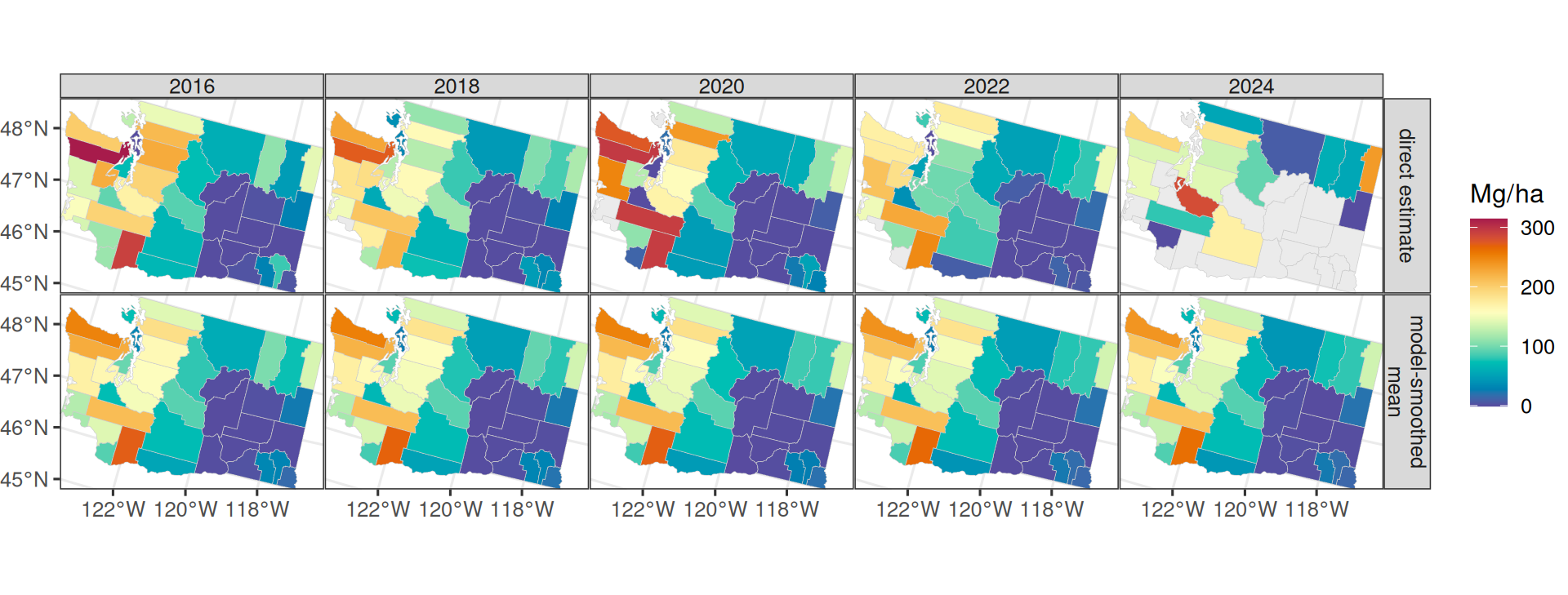
The next figure compares observed direct estimates with model-smoothed county-year means. Counties with no direct estimate in a year can still receive a model-based estimate because their county-year latent effect is part of the CAR-time support.
Show direct-versus-smoothed map code
panel_years <- c(2016, 2018, 2020, 2022, 2024)

map_dat <- wa_counties |>
  left_join(
    county_year_summary |> filter(year %in% panel_years),
    by = "county_fips"
  )

map_long <- bind_rows(
  map_dat |> mutate(quantity = "direct estimate", value = direct_biomass_model),
  map_dat |> mutate(quantity = "model-smoothed\nmean", value = theta_mean)
) |>
  mutate(quantity = factor(quantity, levels = c("direct estimate", "model-smoothed\nmean")))

ggplot(map_long) +
  geom_sf(aes(fill = value), color = "grey80", linewidth = 0.12) +
  coord_sf(expand = FALSE) +
  facet_grid(quantity ~ year) +
  scale_fill_gradientn(
    colors = stlmm_palette(),
    name = "Mg/ha",
    na.value = "grey92"
  ) +
  theme(
    panel.spacing = grid::unit(0.02, "lines"),
    strip.text = element_text(margin = margin(1, 1, 1, 1)),
    plot.margin = margin(0, 0, 0, 0)
  )
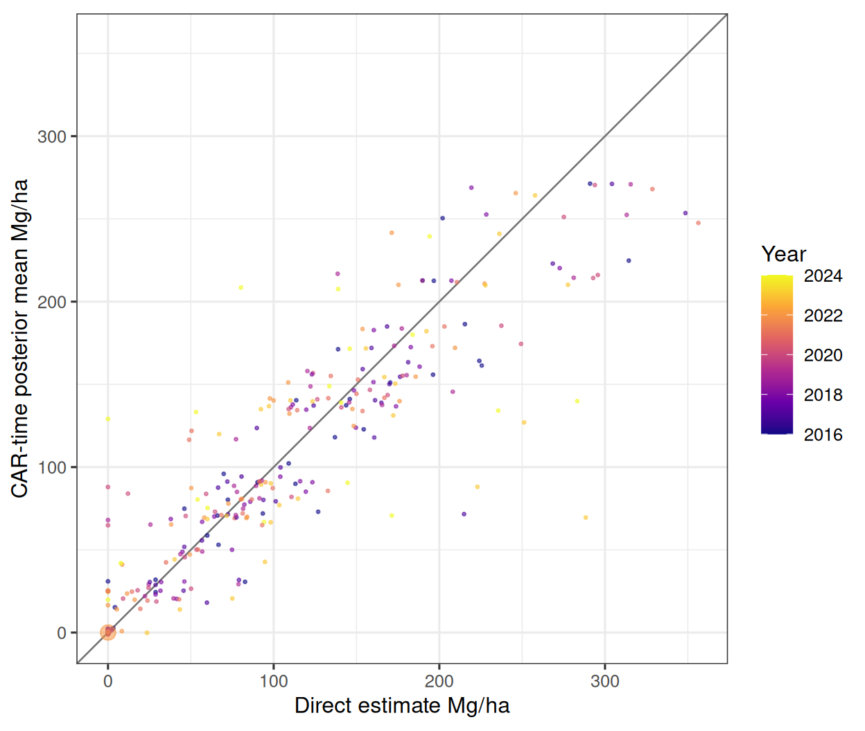
The scatter plot shows the same comparison only for county-years used in the direct-estimate likelihood. The model is not trying to reproduce every noisy direct estimate; it smooths them according to the scaled variance model and the county-time dependence structure.
Show direct-versus-smoothed scatter code
scatter_dat <- county_year_summary |>
  filter(!is.na(direct_biomass_model))

fit_axis_limits <- range(
  c(scatter_dat$direct_biomass_model, scatter_dat$theta_mean, 0),
  na.rm = TRUE
)

ggplot(scatter_dat, aes(x = direct_biomass_model, y = theta_mean)) +
  geom_abline(slope = 1, intercept = 0, color = "grey45", linewidth = 0.45) +
  geom_point(
    aes(size = 1 / direct_biomass_vhat_model, color = year),
    alpha = 0.55
  ) +
  scale_size_continuous(range = c(0.5, 3.5), guide = "none") +
  scale_color_viridis_c(option = "C") +
  coord_equal(xlim = fit_axis_limits, ylim = fit_axis_limits) +
  labs(
    x = "Direct estimate Mg/ha",
    y = "CAR-time posterior mean Mg/ha",
    color = "Year"
  )
9 County Time Series
Time series show how the model smooths through years with sparse or missing direct estimates. The example counties below are selected to include different FIA units and biomass ranges.
Show county time-series code
selected_counties <- c("Clallam", "King", "Okanogan", "Yakima")

series_dat <- county_year_summary |>
  filter(county %in% selected_counties) |>
  mutate(county = factor(county, levels = selected_counties))

ggplot(series_dat, aes(x = year)) +
  geom_ribbon(
    aes(ymin = theta_lower, ymax = theta_upper),
    fill = "#9ecae1",
    alpha = 0.45
  ) +
  geom_line(aes(y = theta_mean), color = stlmm_color("primary"), linewidth = 0.7) +
  geom_point(
    aes(y = direct_biomass_model, size = n),
    color = stlmm_color("secondary"),
    alpha = 0.75,
    na.rm = TRUE
  ) +
  facet_wrap(~ county, ncol = 2, scales = "free_y") +
  scale_x_continuous(breaks = seq(min(series_dat$year), max(series_dat$year), by = 5)) +
  scale_size_continuous(range = c(1, 3.5), name = "Plot n") +
  labs(
    x = "Year",
    y = "Live aboveground biomass Mg/ha"
  )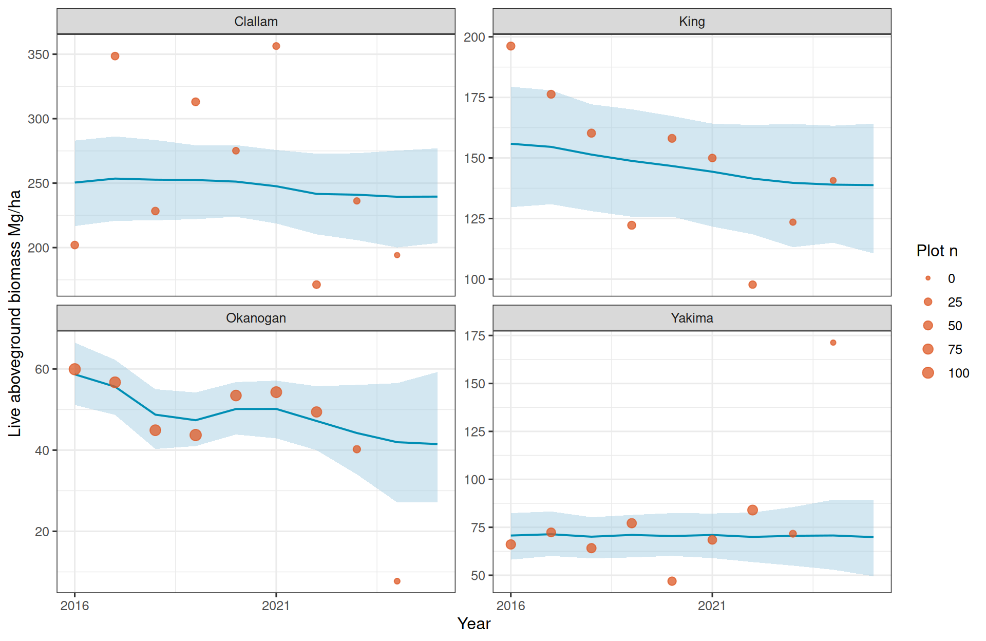
The ribbons are 95% posterior credible intervals for the latent county-year mean. Points are model-ready direct estimates, with point size proportional to the number of FIA plot rows used in that county-year direct estimate. These intervals do not include posterior predictive error for a new direct estimate; the direct-estimate observation variance is represented by the noisy points, not added to the ribbon.
10 TCC and Residual Structure
Adding TCC changes the mean model, not the inferential target. The posterior summaries still describe county-year biomass means, but the model can now use a covariate observed for every county-year before relying on the CAR-time process.
The scaled residual variance model remains a separate part of the hierarchy. The supplied direct-estimate variances still describe relative precision across county-years, but the model estimates how strongly those variances should be trusted. With n_eff_model, lower-sample-size direct estimates shrink more toward a common variance scale, while higher-sample-size direct estimates stay closer to their supplied variance.
If TCC explains broad county-year biomass patterns, the CAR-time process should have less large-scale structure to absorb. The variance scaling parameters do not have to move in a predetermined direction, because they describe observation uncertainty in the direct estimates rather than unexplained mean structure.
WAIC can be used to compare this model with the no-TCC scaled-variance model because both use the same likelihood rows. This article leaves that comparison to a targeted model-assessment analysis so the focus stays on the modeling extension itself.
11 Summary
This article adds the first auxiliary predictor to the area-response workflow:
- the response rows are model-ready county-year direct estimates;
- single-plot county-years remain in the county-year support but do not enter the direct-estimate likelihood;
- county mean TCC enters the latent mean model as a standardized covariate;
- scaled direct-estimate variances enter through
resid(model = "scaled", variance = ..., n = ...); - the county graph defines spatial borrowing;
-
car_time()adds separable county-time smoothing; -
recover()is needed before computing fitted values with Gaussian structured-process models; - the common output is a county-year table of posterior means and 95% credible intervals.
The next area-response article can add spatially varying coefficients or other covariates. That shifts the series from using TCC as a single global mean effect toward asking whether the biomass-TCC relationship changes across the county graph or through time.