
Unit-response BHF model ladder
Plot-level biomass models for the Washington series target
Source:vignettes/wa-unit-bhf-ladder.qmd
1 Purpose
This article opens the unit-response part of the Washington county biomass series. The response is the plot-level agb_live_mg_ha variable, the same variable used to build the simple county-year direct estimates in the area-response articles.
This is a unit-response workflow: the model is fit to FIA plot rows, predictions are made over a county-year grid, and county-year summaries are computed by averaging posterior predictive draws over grid rows. The article uses a short BHF-style ladder (Battese et al. 1988):
- a Gaussian BHF model with row-level TCC, independent county effects, and a shared temporal AR(1) year effect;
- a positive-biomass two-stage model with row-level TCC and shared AR(1) year effects in both stages.
2 Working Target
Let \(j\) index an observed FIA plot row, with county \(a_j\) and measurement year \(t_j\). The plot-level response, \(y_j\), is the agb_live_mg_ha column for row \(j\).
Let \(g\) index a prediction-grid row, with county \(a_g\) and year \(t_g\). For this article, the county-year target is the average agb_live_mg_ha response over the grid rows assigned to county \(a\) and year \(t\),
\[ \theta_{a,t} = \operatorname{avg}_{g \in U_{a,t}} \tilde{y}_g, \]
where \(U_{a,t}\) is the county-year prediction support. In this article, the grid defines the aggregation support for the unit-response summaries. The unobserved grid-row values \(y_g\) are represented by model-based predictions \(\tilde{y}_g\).
The direct estimates in the area-response articles estimate the same kind of mean from observed FIA plot rows,
\[ \hat{y}_{a,t} = \frac{1}{n_{a,t}}\sum_{j \in S_{a,t}} y_j, \]
where \(S_{a,t}\) is the set of observed FIA plot rows in county \(a\) and year \(t\), and \(n_{a,t}\) is the number of rows in that set. As in the overview and area-response articles, \(\hat{y}\) denotes a direct estimate and \(\theta\) denotes the county-year target.
The two-stage model keeps the same target by decomposing agb_live_mg_ha into a binary nonzero indicator and a positive magnitude:
\[ y_j = z_j y_j^+,\qquad z_j = \mathbb{1}(y_j > 0). \]
Here \(y_j^+\) is the positive biomass value when \(y_j > 0\). For posterior prediction, the superscript \((m)\) indexes one retained posterior predictive draw. The two-stage draw for grid row \(g\) is
\[ \tilde{y}_g^{(m)} = \tilde{z}_g^{(m)} \tilde{y}_g^{+,(m)}, \]
and the county-year draw is \(\theta_{a,t}^{(m)} = \operatorname{avg}_{g \in U_{a,t}} \tilde{y}_g^{(m)}\). This is the same hurdle-style product used in the spatial-temporal biomass model of May and Finley (2025), with a binary process for nonzero biomass and a transformed Gaussian model for positive biomass.
3 Data
Show data-reading code
wa_counties <- read_rds(file.path(data_dir, "wa_counties.rds"))
unit_plots <- read_csv(file.path(data_dir, "wa_unit_plots.csv"), show_col_types = FALSE)
direct_estimates <- read_csv(file.path(data_dir, "wa_direct_estimates.csv"), show_col_types = FALSE)
prediction_grid <- read_csv(
  file.path(data_dir, "wa_unit_prediction_grid_10km.csv"),
  show_col_types = FALSE
)

wa_counties <- wa_counties |>
  mutate(county_fips = as.character(county_fips))

unit_plots <- unit_plots |>
  mutate(
    county_fips = as.character(county_fips),
    county_fips = factor(county_fips),
    year = as.integer(year),
    biomass_positive = as.integer(agb_live_mg_ha > 0)
  ) |>
  arrange(county_fips, year, plot_id)

direct_estimates <- direct_estimates |>
  mutate(
    county_fips = as.character(county_fips),
    year = as.integer(year)
  )

plot_years <- sort(unique(unit_plots$year))
tcc_center <- mean(unit_plots$tcc_mean, na.rm = TRUE)
tcc_scale <- sd(unit_plots$tcc_mean, na.rm = TRUE)

unit_plots <- unit_plots |>
  mutate(tcc_mean_scaled = (tcc_mean - tcc_center) / tcc_scale)

county_levels <- levels(unit_plots$county_fips)

prediction_grid <- prediction_grid |>
  mutate(
    county_fips = as.character(county_fips),
    county_fips = factor(county_fips, levels = county_levels),
    year = as.integer(year),
    tcc_mean_scaled = (tcc_mean - tcc_center) / tcc_scale
  ) |>
  filter(year %in% plot_years) |>
  arrange(county_fips, year, x, y)

positive_plots <- unit_plots |>
  filter(biomass_positive == 1) |>
  mutate(biomass_sqrt = sqrt(agb_live_mg_ha))
The plot and grid TCC variables are annual point samples from the USDA Forest Service Tree Canopy Cover raster products (USDA Forest Service 2026). The model uses the same standardization for plot rows and prediction-grid rows, with the center and scale estimated from the observed plot rows.
The article uses the 10 km prediction grid to keep the opening unit-response ladder compact. Later single-model unit-response articles can use the 5 km grid when the focus is on one model rather than a side-by-side ladder.
Show data summary code
data_summary <- tibble(
  quantity = c(
    "plot rows",
    "counties",
    "measurement years",
    "positive-biomass plot rows",
    "zero-biomass plot rows",
    "10 km prediction-grid rows",
    "plot TCC mean",
    "plot TCC SD"
  ),
  value = c(
    fmt_int(nrow(unit_plots)),
    fmt_int(n_distinct(unit_plots$county_fips)),
    paste(range(plot_years), collapse = "-"),
    fmt_int(sum(unit_plots$biomass_positive == 1)),
    fmt_int(sum(unit_plots$biomass_positive == 0)),
    fmt_int(nrow(prediction_grid)),
    fmt_num(tcc_center, 1),
    fmt_num(tcc_scale, 1)
  )
)

show_table(data_summary, caption = "Unit-response data used in the BHF ladder.")| quantity | value |
|---|---|
| plot rows | 6,935 |
| counties | 39 |
| measurement years | 2016-2024 |
| positive-biomass plot rows | 3,991 |
| zero-biomass plot rows | 2,944 |
| 10 km prediction-grid rows | 15,858 |
| plot TCC mean | 41.4 |
| plot TCC SD | 27.9 |
The binned plot below motivates using TCC as the unit-level auxiliary covariate. It is not the model fit; it summarizes how the observed positive-biomass rate and mean square-root positive biomass change across the observed TCC range.
Show TCC binned-response code
tcc_bin_summary <- unit_plots |>
  filter(!is.na(tcc_mean)) |>
  mutate(tcc_bin = ntile(tcc_mean, 10)) |>
  group_by(tcc_bin) |>
  summarise(
    mean_tcc = mean(tcc_mean),
    positive_biomass_rate = mean(biomass_positive),
    mean_sqrt_positive_biomass = mean(
      sqrt(agb_live_mg_ha[biomass_positive == 1]),
      na.rm = TRUE
    ),
    .groups = "drop"
  ) |>
  pivot_longer(
    c(positive_biomass_rate, mean_sqrt_positive_biomass),
    names_to = "quantity",
    values_to = "value"
  ) |>
  mutate(
    quantity = recode(
      quantity,
      positive_biomass_rate = "positive-biomass rate (proportion)",
      mean_sqrt_positive_biomass = "mean sqrt positive biomass"
    )
  )

ggplot(tcc_bin_summary, aes(mean_tcc, value)) +
  geom_line(color = stlmm_color("primary"), linewidth = 0.75) +
  geom_point(color = stlmm_color("secondary"), size = 1.8) +
  facet_wrap(~ quantity, scales = "free_y", ncol = 1) +
  labs(
    x = "mean TCC within observed decile",
    y = "observed binned response"
  ) +
  theme(panel.spacing = grid::unit(0.45, "lines"))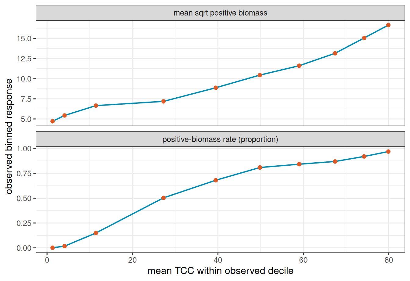
Show year summary code
year_summary <- unit_plots |>
  group_by(year) |>
  summarise(
    plots = n(),
    positive_biomass_rate = mean(biomass_positive),
    mean_response = mean(agb_live_mg_ha),
    median_response = median(agb_live_mg_ha),
    .groups = "drop"
  )

show_table(
  year_summary |>
    filter(year %in% c(2016, 2018, 2020, 2022, 2024)) |>
    mutate(
      positive_biomass_rate = fmt_num(positive_biomass_rate, 2),
      mean_response = fmt_num(mean_response, 1),
      median_response = fmt_num(median_response, 1)
    ),
  caption = "Selected-year summaries of the `agb_live_mg_ha` response."
)| year | plots | positive_biomass_rate | mean_response | median_response |
|---|---|---|---|---|
| 2016 | 991 | 0.60 | 108.9 | 39.9 |
| 2018 | 1020 | 0.59 | 100.2 | 36.5 |
| 2020 | 827 | 0.53 | 104.6 | 15.8 |
| 2022 | 837 | 0.51 | 84.7 | 0.6 |
| 2024 | 86 | 0.51 | 98.7 | 9.0 |
4 Models
The main single-stage model in this article is a Gaussian BHF model with row-level TCC, independent county effects, and a shared AR(1) measurement-year effect:
\[ y_j = \beta_0 + \beta_1 x_j + \alpha_{a_j} + v_{t_j} + e_j, \]
where \(x_j\) is standardized TCC, \(\alpha_a\) is an independent county effect, \(v_t\) follows an AR(1) process over measurement years, and \(e_j\) is residual plot-level variation. The county effect is the BHF area effect. The AR(1) term is common to all counties; it represents shared annual departures, not county-specific time series.
Starting with TCC and a shared AR(1) year effect makes sense for this opening model because the plot rows are not a single cross-section. TCC gives the unit-level model an auxiliary predictor available at both plot and grid rows, while the AR(1) effect adjusts for annual departures shared across Washington. The independent county effect accounts for persistent differences among counties.
That structure is useful for introducing unit-response fitting, prediction, and aggregation, but it is not as flexible as a county-time model. Counties cannot have their own temporally correlated departures beyond the shared year effect and persistent county intercept. The next unit-response CAR-time article will replace this simple structure with a county-year process, so each county can have its own temporal pattern while still borrowing across the county graph.
The two-stage model uses the same temporal idea in both stages. The binary stage models whether agb_live_mg_ha is positive,
\[ z_j \sim \operatorname{bernoulli}(p_j),\qquad \operatorname{logit}(p_j) = \gamma_0 + \gamma_1 x_j + \eta_{a_j} + u_{t_j}, \]
where \(u_t\) follows an AR(1) process over measurement years. For rows with \(y_j > 0\), the positive-biomass stage models the square-root transformed response,
\[ q_j = \sqrt{y_j^+},\qquad q_j = \delta_0 + \delta_1 x_j + \xi_{a_j} + h_{t_j} + r_j,\qquad r_j \sim \operatorname{normal}(0,\tau_+^2). \]
Here \(h_t\) is a second AR(1) year effect for positive biomass. The two stages are fit separately, then recombined draw by draw so the county-year summaries still target the mean of agb_live_mg_ha.
For prediction, squaring returns the positive-stage draw to Mg/ha, so draw \(m\) combines the two stages at prediction-grid row \(g\) as
\[ \tilde{y}_g^{(m)} = \tilde{z}_g^{(m)} \{\tilde{q}_g^{(m)}\}^2. \]
5 Fit
Show MCMC settings
n_samples <- 10000
burnin <- 5000
chains <- 3
n_keep <- 100
posterior_thin <- max(1L, floor((n_samples - burnin) / n_keep))
posterior_sub_sample <- list(start = burnin + 1, thin = posterior_thin)
chain_control <- list(seed = 7, dispersion = 1.5)
warmup_control <- list(batch_length = 25, min_batches = 10)

response_sd <- sd(unit_plots$agb_live_mg_ha, na.rm = TRUE)
sqrt_response_sd <- sd(positive_plots$biomass_sqrt, na.rm = TRUE)

fit_summary_parameters <- list(
  gaussian_ar1 = c(
    "(Intercept)", "tcc_mean_scaled", "tau_sq",
    "iid_1_sigma_sq", "ar1_1_sigma_sq", "ar1_1_phi"
  ),
  positive_ar1 = c(
    "(Intercept)", "tcc_mean_scaled",
    "iid_1_sigma_sq", "ar1_1_sigma_sq", "ar1_1_phi"
  ),
  positive_biomass_ar1 = c(
    "(Intercept)", "tcc_mean_scaled", "tau_sq",
    "iid_1_sigma_sq", "ar1_1_sigma_sq", "ar1_1_phi"
  )
)

select_summary_parameters <- function(x, parameters) {
  keep <- intersect(parameters, rownames(x$parameters))
  x$parameters <- x$parameters[keep, , drop = FALSE]
  if (!is.null(x$diagnostics)) {
    x$diagnostics <- x$diagnostics[x$diagnostics$parameter %in% keep, , drop = FALSE]
  }
  x
}
5.1 Main Gaussian BHF With TCC and Temporal AR(1)
gaussian_ar1_fit <- stLMM(
  agb_live_mg_ha ~ tcc_mean_scaled + iid(county_fips) + ar1(year),
  data = unit_plots,
  priors = list(
    beta = normal(mean = 0, sd = 2 * response_sd),
    resid = list(tau_sq = half_t(df = 3, scale = response_sd)),
    iid_1 = list(sigma_sq = ig(shape = 3, scale = 2 * response_sd^2)),
    ar1_1 = list(
      sigma_sq = half_t(df = 3, scale = response_sd),
      phi = uniform(0.01, 0.99)
    )
  ),
  n_samples = n_samples,
  chains = chains,
  chain_control = chain_control,
  warmup = warmup_control,
  verbose = TRUE,
  n_report = 500
)

gaussian_ar1_summary <- summary(
  gaussian_ar1_fit,
  burn = burnin
) |>
  select_summary_parameters(fit_summary_parameters$gaussian_ar1)
5.2 Positive-Biomass Two-Stage Model With TCC and Temporal AR(1)
positive_ar1_fit <- stLMM(
  biomass_positive ~ tcc_mean_scaled + iid(county_fips) + ar1(year),
  data = unit_plots,
  family = "binomial",
  priors = list(
    beta = normal(mean = 0, sd = 2.5),
    iid_1 = list(sigma_sq = ig(shape = 3, scale = 2)),
    ar1_1 = list(
      sigma_sq = half_t(df = 3, scale = 1),
      phi = uniform(0.01, 0.99)
    )
  ),
  n_samples = n_samples,
  chains = chains,
  chain_control = chain_control,
  warmup = warmup_control,
  verbose = TRUE,
  n_report = 500
)

positive_ar1_summary <- summary(
  positive_ar1_fit,
  burn = burnin
) |>
  select_summary_parameters(fit_summary_parameters$positive_ar1)

positive_biomass_ar1_fit <- stLMM(
  biomass_sqrt ~ tcc_mean_scaled + iid(county_fips) + ar1(year),
  data = positive_plots,
  priors = list(
    beta = normal(mean = 0, sd = 2 * sqrt_response_sd),
    resid = list(tau_sq = half_t(df = 3, scale = sqrt_response_sd)),
    iid_1 = list(sigma_sq = ig(shape = 3, scale = 2 * sqrt_response_sd^2)),
    ar1_1 = list(
      sigma_sq = half_t(df = 3, scale = sqrt_response_sd),
      phi = uniform(0.01, 0.99)
    )
  ),
  n_samples = n_samples,
  chains = chains,
  chain_control = chain_control,
  warmup = warmup_control,
  verbose = TRUE,
  n_report = 500
)

positive_biomass_ar1_summary <- summary(
  positive_biomass_ar1_fit,
  burn = burnin
) |>
  select_summary_parameters(fit_summary_parameters$positive_biomass_ar1)
Show fit summaries
gaussian_ar1_summarystLMM multi-chain summary
formula: agb_live_mg_ha ~ tcc_mean_scaled + iid(county_fips) + ar1(year)
chains: 3
family: gaussian
observations: 6935
posterior draws per chain: 10000 (5000 used after burn = 5000)
process terms: 1
Parameters:
mean sd q2.5 q50.0 q97.5
(Intercept) 97.2751 14.8092 67.8210 97.8262 123.1547
tcc_mean_scaled 96.7532 2.3089 92.2283 96.7539 101.3033
tau_sq 13240.9286 224.2403 12803.6525 13238.9503 13684.1726
iid_1_sigma_sq 3513.6372 819.9498 2271.1592 3394.2842 5431.2728
ar1_1_sigma_sq 183.2147 716.2953 0.1592 37.2177 1347.2310
ar1_1_phi 0.6236 0.2915 0.0567 0.6874 0.9851
Chain diagnostics:
parameter rhat effective_size
(Intercept) (Intercept) 1.0029 2234.3402
tcc_mean_scaled tcc_mean_scaled 1.0003 3358.9732
tau_sq tau_sq 1.0003 1084.0322
iid_1_sigma_sq iid_1_sigma_sq 1.0002 12249.4579
ar1_1_sigma_sq ar1_1_sigma_sq 1.0882 767.6725
ar1_1_phi ar1_1_phi 1.0035 952.1482Show fit summaries
positive_ar1_summarystLMM multi-chain summary
formula: biomass_positive ~ tcc_mean_scaled + iid(county_fips) + ar1(year)
chains: 3
family: binomial
observations: 6935
posterior draws per chain: 10000 (5000 used after burn = 5000)
process terms: 1
Parameters:
mean sd q2.5 q50.0 q97.5
(Intercept) -0.2185 0.4039 -1.0505 -0.2115 0.5209
tcc_mean_scaled 2.6688 0.0729 2.5276 2.6689 2.8097
iid_1_sigma_sq 1.4089 0.3787 0.8455 1.3557 2.3199
ar1_1_sigma_sq 0.3418 0.5592 0.0276 0.1868 1.7232
ar1_1_phi 0.3684 0.2691 0.0212 0.3013 0.9276
Chain diagnostics:
parameter rhat effective_size
(Intercept) (Intercept) 1.0013 6136.1901
tcc_mean_scaled tcc_mean_scaled 1.0014 1671.5420
iid_1_sigma_sq iid_1_sigma_sq 1.0009 2549.9206
ar1_1_sigma_sq ar1_1_sigma_sq 1.0059 875.5614
ar1_1_phi ar1_1_phi 1.0068 1093.3239Show fit summaries
positive_biomass_ar1_summarystLMM multi-chain summary
formula: biomass_sqrt ~ tcc_mean_scaled + iid(county_fips) + ar1(year)
chains: 3
family: gaussian
observations: 3991
posterior draws per chain: 10000 (5000 used after burn = 5000)
process terms: 1
Parameters:
mean sd q2.5 q50.0 q97.5
(Intercept) 9.6660 0.5856 8.5378 9.6732 10.7545
tcc_mean_scaled 3.8453 0.1635 3.5223 3.8457 4.1650
tau_sq 22.5221 0.4987 21.5802 22.5196 23.5511
iid_1_sigma_sq 5.9773 1.5290 3.6989 5.7449 9.5887
ar1_1_sigma_sq 0.2140 0.7575 0.0001 0.0461 1.4380
ar1_1_phi 0.5744 0.2957 0.0431 0.6007 0.9831
Chain diagnostics:
parameter rhat effective_size
(Intercept) (Intercept) 1.0071 1579.8415
tcc_mean_scaled tcc_mean_scaled 1.0003 5408.5871
tau_sq tau_sq 1.0009 1092.7246
iid_1_sigma_sq iid_1_sigma_sq 1.0001 8936.8664
ar1_1_sigma_sq ar1_1_sigma_sq 1.0484 874.5624
ar1_1_phi ar1_1_phi 1.0021 977.7999The fit summaries focus on fixed effects and variance parameters. County-specific random-effect coefficients are omitted from the printed summaries because there are many of them; they should still be checked in diagnostics when fitting the model for inference.
The single-stage Gaussian model estimates the mean of agb_live_mg_ha directly. The two-stage model separates the zero and positive parts while keeping the same county-year target after draw-wise recombination.
6 Prediction and Aggregation
The 10 km grid rows define the county-year prediction support. For each fitted model, posterior predictive draws are averaged over grid rows within each county-year. The Gaussian predictions use y_samples = TRUE, so the aggregated draws include residual predictive uncertainty before county-year averaging.
Show aggregation helper code
prediction_sample_matrix <- function(pred, sample) {
  as.matrix(as_samples(pred, sample = sample, metadata = FALSE))
}

aggregate_grid_draws <- function(draws, grid, prefix = "") {
  county_year <- grid |>
    distinct(county_fips, county, year) |>
    arrange(county_fips, year)

  county_samples <- matrix(
    NA_real_,
    nrow = nrow(draws),
    ncol = nrow(county_year)
  )

  for (j in seq_len(nrow(county_year))) {
    ii <- which(
      grid$county_fips == county_year$county_fips[j] &
        grid$year == county_year$year[j]
    )
    county_samples[, j] <- rowMeans(draws[, ii, drop = FALSE])
  }

  county_year |>
    bind_cols(
      summarize_draw_matrix(county_samples, prefix = prefix) |>
        select(-prediction_row)
    )
}
Structured Gaussian process terms are collapsed during fitting. Models with AR(1) year effects therefore need recover() before prediction.
The summaries below estimate the same series target, but they encode different assumptions about the plot response distribution.
Show summary-combination code
model_summaries <- bind_rows(
  gaussian_ar1_county_summary |> mutate(model = "Gaussian BHF + TCC + AR(1)"),
  two_stage_ar1_county_summary |> mutate(model = "two-stage + TCC + AR(1)")
) |>
  mutate(
    county_fips = as.character(county_fips),
    model = factor(
      model,
      levels = c("Gaussian BHF + TCC + AR(1)", "two-stage + TCC + AR(1)")
    )
  )

direct_for_compare <- direct_estimates |>
  filter(year %in% plot_years) |>
  select(
    county_fips, county, year, n,
    direct_biomass_model, direct_biomass_se_model
  )
Show selected summary table code
show_table(
  model_summaries |>
    filter(year == 2024) |>
    left_join(
      direct_for_compare |> filter(year == 2024),
      by = c("county_fips", "county", "year")
    ) |>
    arrange(model, desc(theta_mean)) |>
    group_by(model) |>
    slice_head(n = 5) |>
    ungroup() |>
    select(model, county, n, direct_biomass_model, theta_mean, theta_lower, theta_upper) |>
    mutate(
      across(
        c(direct_biomass_model, theta_mean, theta_lower, theta_upper),
        ~ fmt_num(.x, 1)
      )
    ),
  caption = "Highest 2024 county-year posterior predictive means by unit-response model."
)| model | county | n | direct_biomass_model | theta_mean | theta_lower | theta_upper |
|---|---|---|---|---|---|---|
| Gaussian BHF + TCC + AR(1) | Skamania | 0 | NA | 267.2 | 225.7 | 299.9 |
| Gaussian BHF + TCC + AR(1) | Clallam | 3 | 194.2 | 243.4 | 208.2 | 282.5 |
| Gaussian BHF + TCC + AR(1) | Jefferson | 2 | 139.0 | 226.8 | 188.6 | 267.2 |
| Gaussian BHF + TCC + AR(1) | Lewis | 3 | 80.3 | 217.3 | 185.8 | 248.3 |
| Gaussian BHF + TCC + AR(1) | Grays Harbor | 3 | 145.9 | 165.6 | 131.2 | 201.4 |
| two-stage + TCC + AR(1) | Skamania | 0 | NA | 246.1 | 190.5 | 303.6 |
| two-stage + TCC + AR(1) | Clallam | 3 | 194.2 | 216.4 | 166.8 | 273.2 |
| two-stage + TCC + AR(1) | Jefferson | 2 | 139.0 | 194.2 | 123.7 | 251.5 |
| two-stage + TCC + AR(1) | Lewis | 3 | 80.3 | 191.7 | 153.4 | 236.0 |
| two-stage + TCC + AR(1) | Grays Harbor | 3 | 145.9 | 155.2 | 111.3 | 201.6 |
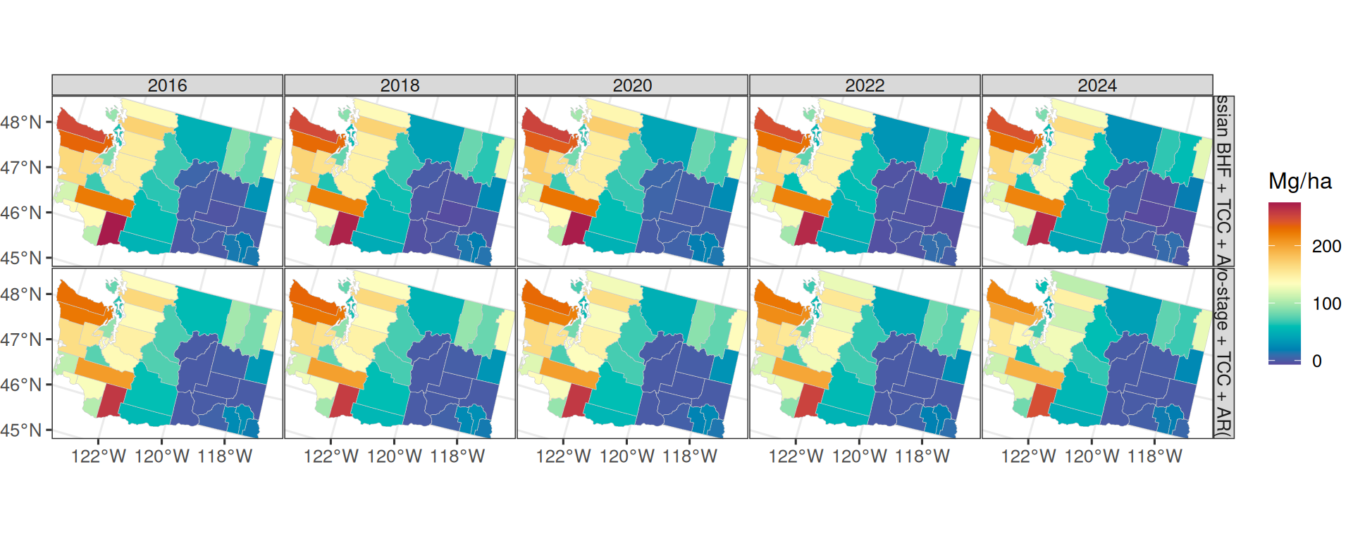
7 Maps
Show prediction map code
panel_years <- c(2016, 2018, 2020, 2022, 2024)

map_dat <- wa_counties |>
  left_join(
    model_summaries |> filter(year %in% panel_years),
    by = "county_fips"
  )

ggplot(map_dat) +
  geom_sf(aes(fill = theta_mean), color = "grey80", linewidth = 0.12) +
  coord_sf(expand = FALSE) +
  facet_grid(model ~ year) +
  scale_fill_gradientn(
    colors = stlmm_palette(),
    name = "Mg/ha",
    na.value = "grey92"
  ) +
  theme(
    panel.spacing = grid::unit(0.03, "lines"),
    strip.text = element_text(margin = margin(1, 1, 1, 1)),
    plot.margin = margin(0, 0, 0, 0)
  )
8 County Time Series
The time-series figure compares direct estimates with the two unit-response summaries for selected counties. Direct estimates are shown only where the county-year had a model-ready direct estimate.
Show county time-series code
profile_counties <- c("Clallam", "King", "Okanogan", "Yakima")

profile_dat <- model_summaries |>
  filter(county %in% profile_counties) |>
  mutate(county = factor(county, levels = profile_counties))

profile_direct <- direct_for_compare |>
  filter(county %in% profile_counties) |>
  mutate(county = factor(county, levels = profile_counties))

ggplot(profile_dat, aes(year, theta_mean, color = model, fill = model)) +
  geom_ribbon(
    aes(ymin = theta_lower, ymax = theta_upper),
    alpha = 0.12,
    color = NA
  ) +
  geom_line(linewidth = 0.75) +
  geom_point(
    data = profile_direct,
    aes(year, direct_biomass_model),
    inherit.aes = FALSE,
    color = "grey20",
    size = 1.4,
    alpha = 0.75
  ) +
  facet_wrap(~ county, scales = "free_y", ncol = 2) +
  scale_color_manual(values = stlmm_discrete_colors(2)) +
  scale_fill_manual(values = stlmm_discrete_colors(2)) +
  labs(
    x = "year",
    y = "mean agb_live_mg_ha (Mg/ha)",
    color = NULL,
    fill = NULL
  ) +
  theme(legend.position = "bottom")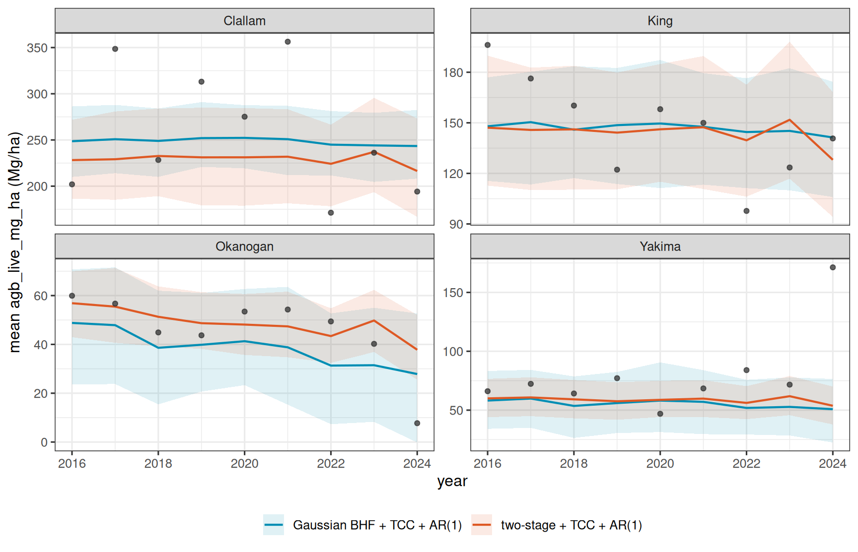
The county panels are a useful check on the unit-response summaries because they show how the single-stage and two-stage models respond to sparse county-year direct estimates. In Yakima, the unit-response summaries are consistently lower than many of the direct estimates. We return to this pattern in the next article, where the model is better matched to the county-time structure in the data and the lower Yakima predictions persist.
9 Takeaways
This ladder starts the unit-response sequence with deliberately simple area effects. The Gaussian TCC plus AR(1) model is the single-stage baseline because it keeps the BHF county effect, uses a grid-available auxiliary covariate, and adds shared temporal borrowing across measurement years. The two-stage model addresses the zero-inflated response while preserving the same series target through draw-wise products. These models are useful starting points for the software workflow, but they are less flexible than the county-time models that follow.
The next unit-response article moves directly to a two-stage county-time CAR model with row-level TCC. A later unit-response article can add FIA-unit-specific residual variance in the positive Gaussian stage, followed by a continuous space-time model.