
Unit-response two-stage CAR-time model with FIA-unit variances
A residual-variance refinement for Washington biomass
Source:vignettes/wa-unit-two-stage-car-time-tcc-fiaunit-var.qmd
1 Purpose
This article keeps the same two-stage CAR-time TCC mean model from the previous unit-response article and changes only the positive-biomass residual variance. The binary stage still models agb_live_mg_ha > 0; the positive stage still models square-root positive agb_live_mg_ha; and the county-year target remains the grid-supported mean of agb_live_mg_ha.
The variance refinement is useful because Washington counties span large biomass gradients, from relatively low-biomass dry interior forests to high-biomass coastal and western forests. A common residual variance asks the positive-biomass model to use one plot-level noise scale across that full range. Allowing the residual variance to differ by FIA unit gives the positive stage a simple way to accommodate broad heteroskedasticity while leaving the occurrence model, mean structure, and aggregation target unchanged.
The extension is
\[ q_j = \delta_0 + \delta_1 x_j + w^+_{a_j,t_j} + r_j,\qquad r_j \sim \operatorname{normal}(0,\tau^2_{u_j}), \]
where \(q_j = \sqrt{y_j^+}\), \(x_j\) is standardized row-level TCC, \(w^+_{a,t}\) is the positive-stage CAR-time process, and \(u_j\) is the FIA unit for plot row \(j\). This is a variance-model refinement, not a new estimand or a new mean structure.
2 Data
Show data-reading code
wa_counties <- read_rds(file.path(data_dir, "wa_counties.rds"))
unit_plots <- read_csv(file.path(data_dir, "wa_unit_plots.csv"), show_col_types = FALSE)
direct_estimates <- read_csv(file.path(data_dir, "wa_direct_estimates.csv"), show_col_types = FALSE)
prediction_grid <- read_csv(
  file.path(data_dir, "wa_unit_prediction_grid_5km.csv"),
  show_col_types = FALSE
)

wa_counties <- wa_counties |>
  mutate(
    county_fips = as.character(county_fips),
    fia_unit = factor(fia_unit)
  )

unit_plots <- unit_plots |>
  mutate(
    county_fips = as.character(county_fips),
    county_fips = factor(county_fips),
    fia_unit = factor(fia_unit),
    year = as.integer(year),
    biomass_positive = as.integer(agb_live_mg_ha > 0)
  ) |>
  arrange(county_fips, year, plot_id)

direct_estimates <- direct_estimates |>
  mutate(
    county_fips = as.character(county_fips),
    year = as.integer(year)
  )

plot_years <- sort(unique(unit_plots$year))
tcc_center <- mean(unit_plots$tcc_mean, na.rm = TRUE)
tcc_scale <- sd(unit_plots$tcc_mean, na.rm = TRUE)

unit_plots <- unit_plots |>
  mutate(tcc_mean_scaled = (tcc_mean - tcc_center) / tcc_scale)

county_levels <- levels(unit_plots$county_fips)
fia_unit_levels <- levels(unit_plots$fia_unit)
fia_unit_names <- unit_plots |>
  distinct(fia_unit, fia_unit_name) |>
  arrange(fia_unit)

prediction_grid <- prediction_grid |>
  mutate(
    county_fips = as.character(county_fips),
    county_fips = factor(county_fips, levels = county_levels),
    fia_unit = factor(fia_unit, levels = fia_unit_levels),
    year = as.integer(year),
    tcc_mean_scaled = (tcc_mean - tcc_center) / tcc_scale
  ) |>
  filter(year %in% plot_years) |>
  arrange(county_fips, year, x, y)

positive_plots <- unit_plots |>
  filter(biomass_positive == 1) |>
  mutate(biomass_sqrt = sqrt(agb_live_mg_ha))
The plot and grid TCC variables are annual point samples from the USDA Forest Service Tree Canopy Cover raster products (USDA Forest Service 2026). This article uses the same plot-based TCC standardization and 5 km prediction support as the previous two-stage CAR-time TCC article.
Show data summary code
data_summary <- tibble(
  quantity = c(
    "plot rows",
    "positive-biomass plot rows",
    "FIA units",
    "5 km prediction-grid rows"
  ),
  value = c(
    fmt_int(nrow(unit_plots)),
    fmt_int(nrow(positive_plots)),
    fmt_int(n_distinct(unit_plots$fia_unit)),
    fmt_int(nrow(prediction_grid))
  )
)

show_table(data_summary, caption = "Unit-response data for the FIA-unit variance model.")| quantity | value |
|---|---|
| plot rows | 6,935 |
| positive-biomass plot rows | 3,991 |
| FIA units | 5 |
| 5 km prediction-grid rows | 63,306 |
3 County Graph
The CAR-time mean structure is unchanged from the previous article.
g <- car_graph(
  wa_counties,
  id = "county_fips",
  island = "nearest",
  island_k = 4
)

g$island_added_edges
from to distance
1 53055 53029 56295.37
2 53055 53035 100453.91
3 53055 53073 100817.65
4 53055 53057 102288.114 Fit
Only the positive-biomass stage changes. The binary occurrence stage is the same Bernoulli CAR-time TCC model used in the previous article.
Show MCMC settings
n_samples <- 10000
burnin <- 5000
chains <- 3
n_keep <- 100
posterior_thin <- max(1L, floor((n_samples - burnin) / n_keep))
posterior_sub_sample <- list(start = burnin + 1, thin = posterior_thin)
chain_control <- list(seed = 17, dispersion = 1.5)
warmup_control <- list(batch_length = 25, min_batches = 10)

sqrt_response_sd <- sd(positive_plots$biomass_sqrt, na.rm = TRUE)
occurrence_fit <- stLMM(
  biomass_positive ~
    tcc_mean_scaled +
    car_time(county_fips, year, graph = g, car_model = "leroux"),
  data = unit_plots,
  family = "binomial",
  priors = list(
    beta = normal(mean = 0, sd = 2.5),
    car_time_1 = list(
      sigma_sq = half_t(df = 3, scale = 1),
      rho = uniform(0.01, 0.99),
      phi = uniform(-0.99, 0.99)
    )
  ),
  n_samples = n_samples,
  chains = chains,
  chain_control = chain_control,
  warmup = warmup_control,
  verbose = TRUE,
  n_report = 500
)
biomass_fit <- stLMM(
  biomass_sqrt ~
    tcc_mean_scaled +
    car_time(county_fips, year, graph = g, car_model = "leroux") +
    resid(model = "group", group = fia_unit),
  data = positive_plots,
  priors = list(
    beta = normal(mean = 0, sd = 2 * sqrt_response_sd),
    resid = list(tau_sq = half_t(df = 3, scale = sqrt_response_sd)),
    car_time_1 = list(
      sigma_sq = half_t(df = 3, scale = sqrt_response_sd),
      rho = uniform(0.01, 0.99),
      phi = uniform(-0.99, 0.99)
    )
  ),
  n_samples = n_samples,
  chains = chains,
  chain_control = chain_control,
  warmup = warmup_control,
  verbose = TRUE,
  n_report = 500
)
Show fit summaries
occurrence_summarystLMM multi-chain summary
formula: biomass_positive ~ tcc_mean_scaled + car_time(county_fips, year, graph = g, car_model = "leroux")
chains: 3
family: binomial
observations: 6935
posterior draws per chain: 10000 (5000 used after burn = 5000)
process terms: 1
Parameters:
mean sd q2.5 q50.0 q97.5
(Intercept) -0.1260 0.7428 -1.7529 -0.1138 1.4560
tcc_mean_scaled 2.7041 0.0738 2.5603 2.7035 2.8493
car_time_1_sigma_sq 3.1468 1.0779 1.5006 3.0051 5.7391
car_time_1_rho 0.6125 0.2632 0.1143 0.6133 0.9836
car_time_1_phi 0.9792 0.0102 0.9520 0.9819 0.9897
Chain diagnostics:
parameter rhat effective_size
(Intercept) (Intercept) 1.0034 14631.3546
tcc_mean_scaled tcc_mean_scaled 1.0005 3671.0478
car_time_1_sigma_sq car_time_1_sigma_sq 1.0045 641.7753
car_time_1_rho car_time_1_rho 1.0030 498.1799
car_time_1_phi car_time_1_phi 1.0046 861.0874Show fit summaries
biomass_summarystLMM multi-chain summary
formula: biomass_sqrt ~ tcc_mean_scaled + car_time(county_fips, year, graph = g, car_model = "leroux") + resid(model = "group", group = fia_unit)
chains: 3
family: gaussian
observations: 3991
posterior draws per chain: 10000 (5000 used after burn = 5000)
process terms: 1
Parameters:
mean sd q2.5 q50.0 q97.5
(Intercept) 9.5629 0.4624 8.6112 9.5726 10.4463
tcc_mean_scaled 3.9556 0.1446 3.6703 3.9560 4.2403
tau_sq_9 13.4495 0.6813 12.2143 13.4172 14.8609
tau_sq_8 14.2661 0.5797 13.1827 14.2505 15.4449
tau_sq_6 30.4992 1.8060 27.2803 30.4147 34.3475
tau_sq_7 30.3226 1.5755 27.2976 30.3068 33.5593
tau_sq_5 31.4626 1.6167 28.5691 31.3531 34.8669
car_time_1_sigma_sq 3.3403 1.1897 1.5610 3.1316 6.2786
car_time_1_rho 0.4275 0.2135 0.0534 0.4189 0.8420
car_time_1_phi 0.9677 0.0198 0.9166 0.9729 0.9890
Chain diagnostics:
parameter rhat effective_size
(Intercept) (Intercept) 1.0015 13887.5301
tcc_mean_scaled tcc_mean_scaled 1.0001 10739.1176
tau_sq_9 tau_sq_9 1.0080 668.3089
tau_sq_8 tau_sq_8 1.0043 634.6008
tau_sq_6 tau_sq_6 1.0036 635.0644
tau_sq_7 tau_sq_7 1.0063 687.9759
tau_sq_5 tau_sq_5 1.0045 696.9316
car_time_1_sigma_sq car_time_1_sigma_sq 1.0028 493.2111
car_time_1_rho car_time_1_rho 1.0070 287.0937
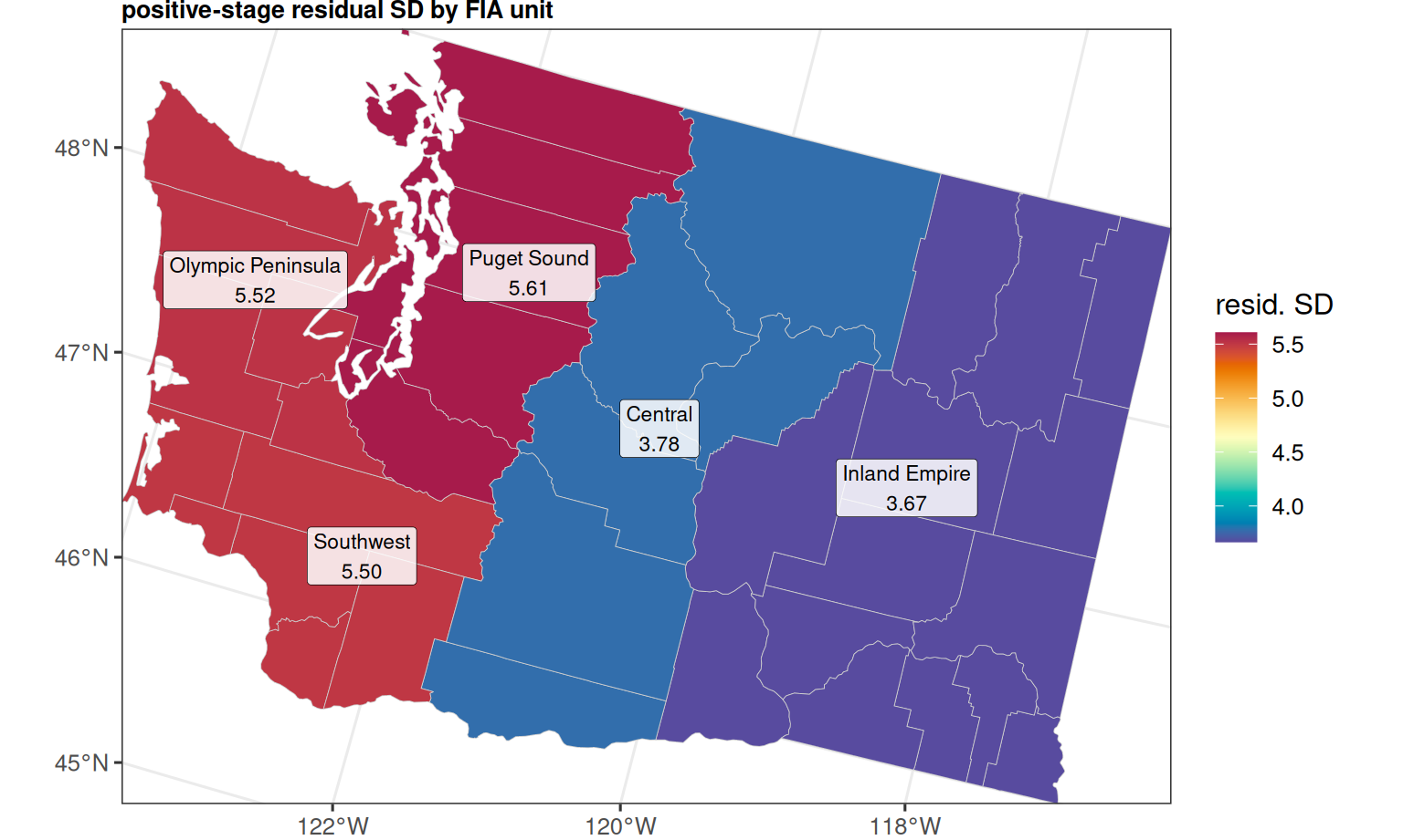
car_time_1_phi car_time_1_phi 1.0077 763.7668The positive-stage summary now includes one residual variance parameter for each FIA unit. The map below shows the corresponding residual standard deviations on the square-root biomass scale.
Show FIA-unit residual SD map code
biomass_draws <- as_samples(biomass_fit, burn = burnin, metadata = FALSE)
resid_var_names <- paste0("tau_sq_", fia_unit_levels)
if (!all(resid_var_names %in% colnames(biomass_draws))) {
  resid_var_names <- fia_unit_levels
}
resid_var_draws <- biomass_draws[, resid_var_names, drop = FALSE]
resid_sd_draws <- sqrt(resid_var_draws)

fia_resid_sd <- tibble(
  fia_unit = factor(fia_unit_levels, levels = fia_unit_levels),
  sd_mean = colMeans(resid_sd_draws),
  sd_lower = apply(resid_sd_draws, 2, quantile, probs = 0.025),
  sd_upper = apply(resid_sd_draws, 2, quantile, probs = 0.975)
) |>
  left_join(fia_unit_names, by = "fia_unit")

fia_resid_map <- wa_counties |>
  select(-fia_unit_name) |>
  left_join(fia_resid_sd, by = "fia_unit")

fia_resid_labels <- fia_resid_map |>
  group_by(fia_unit, fia_unit_name, sd_mean) |>
  summarise(geometry = sf::st_union(geometry), .groups = "drop") |>
  mutate(label = paste0(fia_unit_name, "\n", fmt_num(sd_mean, 2))) |>
  sf::st_point_on_surface()

ggplot(fia_resid_map) +
  geom_sf(aes(fill = sd_mean), color = "grey80", linewidth = 0.15) +
  geom_sf_label(
    data = fia_resid_labels,
    aes(label = label),
    size = 3,
    label.size = 0.12,
    fill = "white",
    alpha = 0.85
  ) +
  coord_sf(expand = FALSE) +
  scale_fill_gradientn(
    colors = stlmm_palette(),
    name = "resid. SD",
    na.value = "grey92"
  ) +
  labs(
    title = "positive-stage residual SD by FIA unit",
    x = NULL,
    y = NULL
  ) +
  theme(
    plot.title = element_text(size = 10, face = "bold", margin = margin(0, 0, 2, 0)),
    plot.margin = margin(0, 0, 0, 0)
  )
Show FIA-unit residual SD table code
show_table(
  fia_resid_sd |>
    transmute(
      `FIA unit` = fia_unit_name,
      `posterior mean SD` = fmt_num(sd_mean, 2),
      `lower` = fmt_num(sd_lower, 2),
      `upper` = fmt_num(sd_upper, 2)
    ),
  caption = "FIA-unit residual standard deviations for square-root positive biomass."
)| FIA unit | posterior mean SD | lower | upper |
|---|---|---|---|
| Puget Sound | 5.61 | 5.35 | 5.90 |
| Olympic Peninsula | 5.52 | 5.22 | 5.86 |
| Southwest | 5.50 | 5.22 | 5.79 |
| Central | 3.78 | 3.63 | 3.93 |
| Inland Empire | 3.67 | 3.49 | 3.85 |
5 Prediction and Aggregation
Prediction is unchanged: draw-wise occurrence predictions are multiplied by squared positive-biomass predictions, then averaged within county-year. The Gaussian positive-stage predictions use y_samples = TRUE, so the squared positive-biomass draws include residual predictive uncertainty before recombination.
Show aggregation helper code
prediction_sample_matrix <- function(pred, sample) {
  as.matrix(as_samples(pred, sample = sample, metadata = FALSE))
}

aggregate_grid_draws <- function(draws, grid, prefix = "") {
  county_year <- grid |>
    distinct(county_fips, county, year) |>
    arrange(county_fips, year)

  county_samples <- matrix(
    NA_real_,
    nrow = nrow(draws),
    ncol = nrow(county_year)
  )

  for (j in seq_len(nrow(county_year))) {
    ii <- which(
      grid$county_fips == county_year$county_fips[j] &
        grid$year == county_year$year[j]
    )
    county_samples[, j] <- rowMeans(draws[, ii, drop = FALSE])
  }

  county_year |>
    bind_cols(
      summarize_draw_matrix(county_samples, prefix = prefix) |>
        select(-prediction_row)
    )
}Show direct-estimate join code
direct_for_compare <- direct_estimates |>
  filter(year %in% plot_years) |>
  select(
    county_fips, county, year, n,
    direct_biomass_model, direct_biomass_se_model
  )

county_summary <- county_summary |>
  mutate(county_fips = as.character(county_fips)) |>
  left_join(
    direct_for_compare,
    by = c("county_fips", "county", "year")
  )
Show selected county-year summary code
show_table(
  county_summary |>
    filter(year == 2024) |>
    arrange(desc(theta_mean)) |>
    select(county, n, direct_biomass_model, theta_mean, theta_lower, theta_upper) |>
    slice_head(n = 10) |>
    mutate(
      across(
        c(direct_biomass_model, theta_mean, theta_lower, theta_upper),
        ~ fmt_num(.x, 1)
      )
    ),
  caption = "Highest 2024 county-year posterior predictive means from the FIA-unit variance model."
)| county | n | direct_biomass_model | theta_mean | theta_lower | theta_upper |
|---|---|---|---|---|---|
| Skamania | 0 | NA | 262.0 | 215.6 | 309.7 |
| Clallam | 3 | 194.2 | 232.6 | 172.2 | 287.4 |
| Jefferson | 2 | 139.0 | 203.1 | 144.9 | 260.1 |
| Lewis | 3 | 80.3 | 194.6 | 158.7 | 233.4 |
| Skagit | 5 | 183.8 | 178.7 | 141.0 | 214.0 |
| Grays Harbor | 3 | 145.9 | 176.1 | 135.1 | 218.3 |
| Mason | 1 | NA | 162.9 | 120.6 | 210.3 |
| Cowlitz | 2 | 0.0 | 148.5 | 106.3 | 192.1 |
| Pacific | 1 | NA | 142.7 | 94.6 | 192.5 |
| King | 7 | 140.7 | 132.5 | 101.4 | 168.4 |
Show county time-series code
profile_counties <- c("Clallam", "King", "Okanogan", "Yakima")

profile_dat <- county_summary |>
  filter(county %in% profile_counties) |>
  mutate(county = factor(county, levels = profile_counties))

ggplot(profile_dat, aes(year, theta_mean)) +
  geom_ribbon(
    aes(ymin = theta_lower, ymax = theta_upper),
    fill = stlmm_color("primary"),
    alpha = 0.15,
    color = NA
  ) +
  geom_line(color = stlmm_color("primary"), linewidth = 0.75) +
  geom_point(
    aes(y = direct_biomass_model),
    color = "grey20",
    size = 1.4,
    alpha = 0.75,
    na.rm = TRUE
  ) +
  facet_wrap(~ county, scales = "free_y", ncol = 2) +
  labs(
    x = "year",
    y = "mean agb_live_mg_ha (Mg/ha)"
  )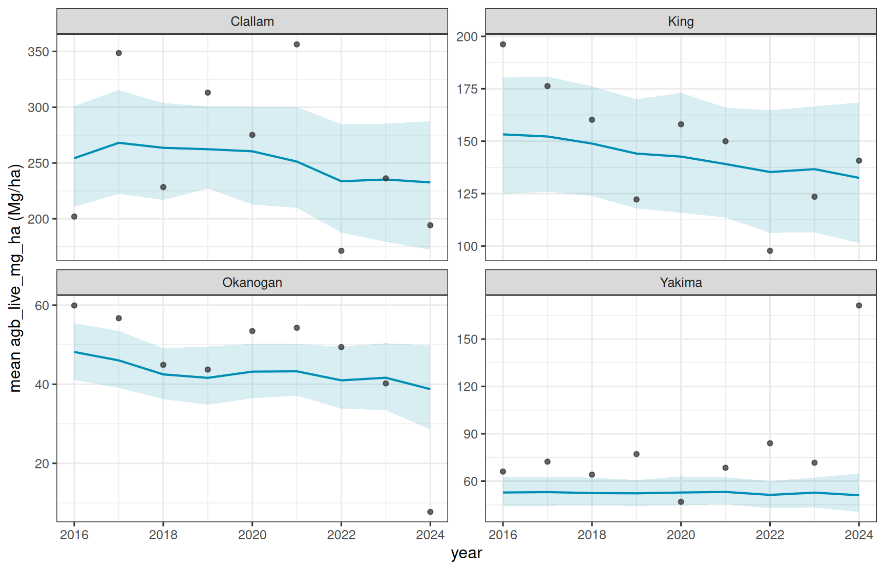
Compared with the previous common-variance model, Okanogan is shifted downward in this figure. Okanogan belongs to the Central FIA unit, which has a smaller estimated positive-stage residual variance than the pooled residual variance used in the previous article. Because the positive stage is fit on the square-root scale and predictions are squared to return to Mg/ha, this residual variance contributes to the back-transformed positive-biomass mean. A smaller residual variance therefore lowers the recombined county-year mean even when the fitted mean structure changes little.
The direct estimates remain a point of comparison, not the model target. This pattern shows what the variance refinement is doing to the model-based grid summary; it does not by itself imply that the grouped-variance model is worse because it is farther from some direct estimates.
6 Takeaways
This article changes the residual variance model, not the target or the mean structure. FIA-unit-specific residual variances let the positive Gaussian stage represent different amounts of plot-level spread across broad FIA units while keeping the same occurrence model, TCC effect, and county-time process.
The main diagnostic is whether the grouped residual SDs differ enough to matter and whether the county-year predictions remain consistent with the previous two-stage CAR-time TCC article.