
Unit-response two-stage CAR-time model with TCC
Plot-level Washington biomass prediction with county-time structure
Source:vignettes/wa-unit-two-stage-car-time-tcc.qmd
1 Purpose
This article continues the unit-response part of the Washington county biomass series. The opening unit-response article introduced BHF-style models with row-level TCC, county effects, and a shared AR(1) year effect. Here the model replaces that simple county-plus-year structure with a county-year effect, so each county can have its own temporal departure while still borrowing across the county graph.
The response is the plot-level agb_live_mg_ha variable used throughout the series. To respect the point mass at zero, the model is two-stage from the start:
- a Bernoulli model for
agb_live_mg_ha > 0; - a Gaussian model for square-root transformed positive
agb_live_mg_ha.
Both stages include row-level tree canopy cover (TCC) and a separable county-year CAR-time process. This keeps the model aligned with the same series target used in the area-response articles, while giving the unit-response model a more useful spatial-temporal structure. The two-stage product follows the same general hurdle-style strategy used in related forest-biomass models (Finley et al. 2011; May and Finley 2025).
2 Working Target
Let \(j\) index an observed FIA plot row, with county \(a_j\), measurement year \(t_j\), and standardized row-level TCC covariate \(x_j\). The plot-level response is \(y_j =\) agb_live_mg_ha.
The county-year target is the mean of agb_live_mg_ha over grid rows assigned to county \(a\) and year \(t\). Let \(g\) index those grid rows. The model predicts \(\tilde{y}_g\) on the original Mg/ha scale and averages posterior predictive draws over grid rows within each county-year.
For equivalence with the area-response direct estimates in this series, the two-stage decomposition is based on agb_live_mg_ha itself,
\[ y_j = z_j y_j^+,\qquad z_j = \mathbb{1}(y_j > 0), \]
where \(y_j^+\) is the positive biomass value for rows with \(y_j > 0\).
The binary stage is
\[ z_j \sim \operatorname{bernoulli}(p_j),\qquad \operatorname{logit}(p_j) = \gamma_0 + \gamma_1 x_j + w^z_{a_j,t_j}, \]
where \(w^z_{a,t}\) is a separable CAR-time process over counties and years. The positive-biomass stage models the square root of positive agb_live_mg_ha,
\[ q_j = \sqrt{y_j^+},\qquad q_j = \delta_0 + \delta_1 x_j + w^+_{a_j,t_j} + r_j,\qquad r_j \sim \operatorname{normal}(0,\tau_+^2), \]
where \(w^+_{a,t}\) is a second CAR-time process for the positive biomass magnitude. The two stages are fit separately and recombined after prediction.
For posterior prediction, superscript \((m)\) indexes one retained posterior predictive draw. The grid-row response draw is
\[ \tilde{y}_g^{(m)} = \tilde{z}_g^{(m)} \left\{\tilde{q}_g^{(m)}\right\}^2, \]
and the county-year draw is obtained by averaging these grid-row draws within county \(a\) and year \(t\).
3 Data
The plot and grid TCC variables are annual point samples from the USDA Forest Service Tree Canopy Cover raster products (USDA Forest Service 2026). The model uses the same standardization for plot rows and prediction-grid rows, with the center and scale estimated from the observed plot rows.
Show data-reading code
wa_counties <- read_rds(file.path(data_dir, "wa_counties.rds"))
unit_plots <- read_csv(file.path(data_dir, "wa_unit_plots.csv"), show_col_types = FALSE)
direct_estimates <- read_csv(file.path(data_dir, "wa_direct_estimates.csv"), show_col_types = FALSE)
prediction_grid <- read_csv(
  file.path(data_dir, "wa_unit_prediction_grid_5km.csv"),
  show_col_types = FALSE
)

wa_counties <- wa_counties |>
  mutate(county_fips = as.character(county_fips))

unit_plots <- unit_plots |>
  mutate(
    county_fips = as.character(county_fips),
    county_fips = factor(county_fips),
    fia_unit = factor(fia_unit),
    year = as.integer(year),
    biomass_positive = as.integer(agb_live_mg_ha > 0)
  ) |>
  arrange(county_fips, year, plot_id)

direct_estimates <- direct_estimates |>
  mutate(
    county_fips = as.character(county_fips),
    year = as.integer(year)
  )

plot_years <- sort(unique(unit_plots$year))
tcc_center <- mean(unit_plots$tcc_mean, na.rm = TRUE)
tcc_scale <- sd(unit_plots$tcc_mean, na.rm = TRUE)

unit_plots <- unit_plots |>
  mutate(tcc_mean_scaled = (tcc_mean - tcc_center) / tcc_scale)

county_levels <- levels(unit_plots$county_fips)
fia_unit_levels <- levels(unit_plots$fia_unit)

prediction_grid <- prediction_grid |>
  mutate(
    county_fips = as.character(county_fips),
    county_fips = factor(county_fips, levels = county_levels),
    fia_unit = factor(fia_unit, levels = fia_unit_levels),
    year = as.integer(year),
    tcc_mean_scaled = (tcc_mean - tcc_center) / tcc_scale
  ) |>
  filter(year %in% plot_years) |>
  arrange(county_fips, year, x, y)

positive_plots <- unit_plots |>
  filter(biomass_positive == 1) |>
  mutate(biomass_sqrt = sqrt(agb_live_mg_ha))
The 5 km grid is the prediction support for this single-model unit-response article. The 10 km grid remains useful for fast local checks.
Show data summary code
data_summary <- tibble(
  quantity = c(
    "plot rows",
    "counties",
    "measurement years",
    "positive-biomass plot rows",
    "zero-biomass plot rows",
    "5 km prediction-grid rows",
    "plot TCC mean",
    "plot TCC SD"
  ),
  value = c(
    fmt_int(nrow(unit_plots)),
    fmt_int(n_distinct(unit_plots$county_fips)),
    paste(range(plot_years), collapse = "-"),
    fmt_int(sum(unit_plots$biomass_positive == 1)),
    fmt_int(sum(unit_plots$biomass_positive == 0)),
    fmt_int(nrow(prediction_grid)),
    fmt_num(tcc_center, 1),
    fmt_num(tcc_scale, 1)
  )
)

show_table(data_summary, caption = "Unit-response data for the two-stage CAR-time TCC model.")| quantity | value |
|---|---|
| plot rows | 6,935 |
| counties | 39 |
| measurement years | 2016-2024 |
| positive-biomass plot rows | 3,991 |
| zero-biomass plot rows | 2,944 |
| 5 km prediction-grid rows | 63,306 |
| plot TCC mean | 41.4 |
| plot TCC SD | 27.9 |
4 County Graph
The county graph defines the spatial component of both CAR-time processes. Washington has island components, so the graph construction adds nearest-neighbor bridge edges.
g <- car_graph(
  wa_counties,
  id = "county_fips",
  island = "nearest",
  island_k = 4
)

g$island_added_edges
from to distance
1 53055 53029 56295.37
2 53055 53035 100453.91
3 53055 53073 100817.65
4 53055 53057 102288.11The figure checks the graph visually. Thin lines connect neighboring county centroids; thicker colored lines show bridge edges added for island components.
Show graph plotting code
coord_dat <- data.frame(
  county_fips = wa_counties$county_fips,
  sf::st_coordinates(sf::st_point_on_surface(sf::st_geometry(wa_counties)))
)

edge_index <- which(as.matrix(g$adjacency) != 0, arr.ind = TRUE)
edge_index <- edge_index[edge_index[, "row"] < edge_index[, "col"], , drop = FALSE]
edge_dat <- tibble(
  from = g$ids[edge_index[, "row"]],
  to = g$ids[edge_index[, "col"]]
) |>
  mutate(
    key = paste(pmin(from, to), pmax(from, to), sep = "--"),
    x = coord_dat$X[match(from, coord_dat$county_fips)],
    y = coord_dat$Y[match(from, coord_dat$county_fips)],
    xend = coord_dat$X[match(to, coord_dat$county_fips)],
    yend = coord_dat$Y[match(to, coord_dat$county_fips)]
  )

island_key <- paste(
  pmin(g$island_added_edges$from, g$island_added_edges$to),
  pmax(g$island_added_edges$from, g$island_added_edges$to),
  sep = "--"
)
edge_dat$island <- edge_dat$key %in% island_key

ggplot(wa_counties) +
  geom_sf(fill = "grey96", color = "white", linewidth = 0.15) +
  geom_segment(
    data = edge_dat,
    aes(x = x, y = y, xend = xend, yend = yend, color = island, linewidth = island)
  ) +
  geom_point(data = coord_dat, aes(X, Y), color = stlmm_color("primary"), size = 1.3) +
  coord_sf(expand = FALSE) +
  scale_color_manual(
    values = c("FALSE" = "grey45", "TRUE" = stlmm_color("secondary")),
    guide = "none"
  ) +
  scale_linewidth_manual(values = c("FALSE" = 0.25, "TRUE" = 1), guide = "none") +
  theme(plot.margin = margin(0, 0, 0, 0))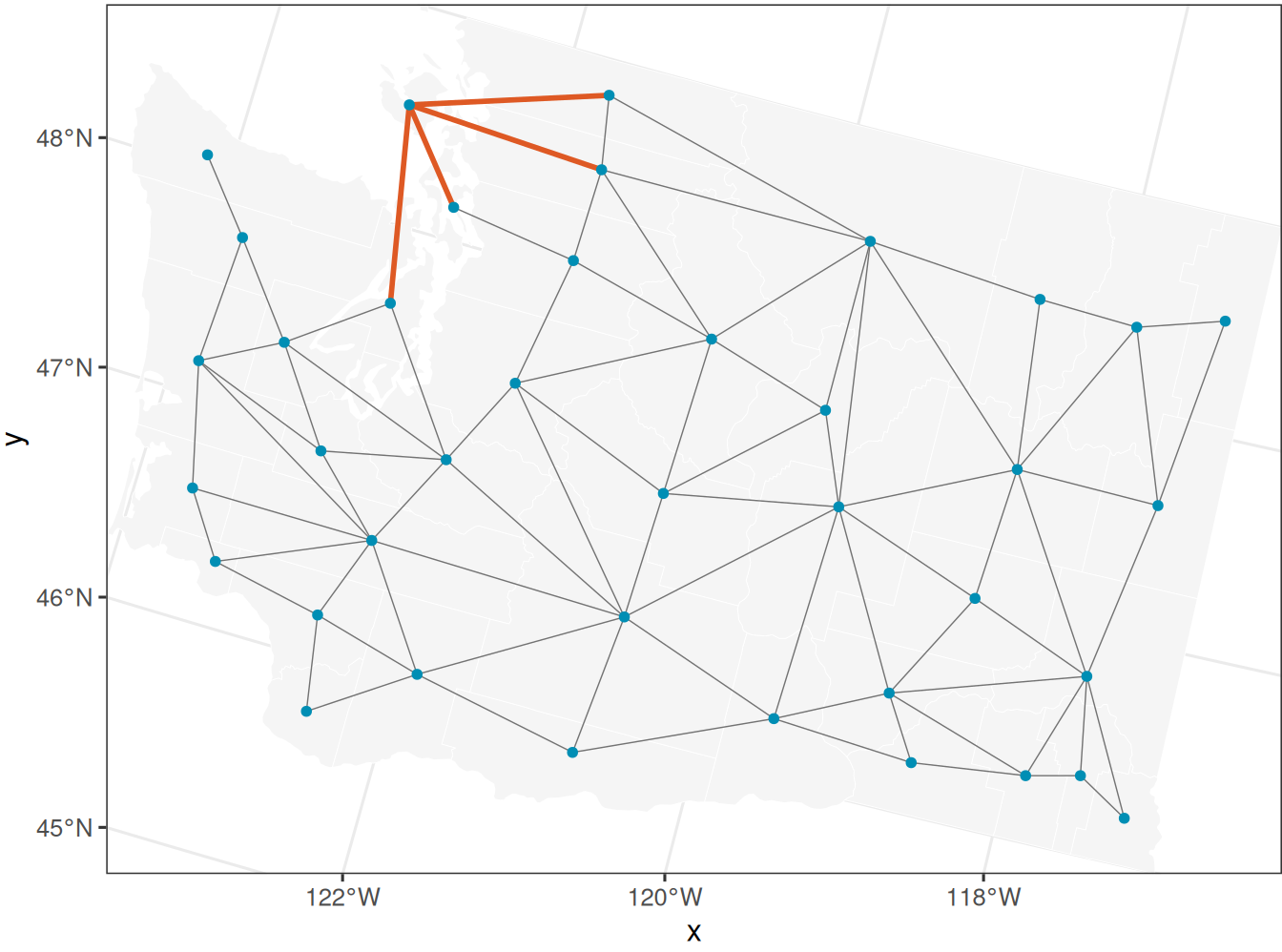
5 Fit
This article fits one unit-response model, but the model has two likelihood stages. The binary stage and positive-biomass stage have separate fixed effects and separate CAR-time processes.
Show MCMC settings
n_samples <- 10000
burnin <- 5000
chains <- 3
n_keep <- 100
posterior_thin <- max(1L, floor((n_samples - burnin) / n_keep))
posterior_sub_sample <- list(start = burnin + 1, thin = posterior_thin)
chain_control <- list(seed = 13, dispersion = 1.5)
warmup_control <- list(batch_length = 25, min_batches = 10)

sqrt_response_sd <- sd(positive_plots$biomass_sqrt, na.rm = TRUE)

fit_summary_parameters <- list(
  occurrence = c(
    "(Intercept)", "tcc_mean_scaled",
    "car_time_1_sigma_sq", "car_time_1_rho", "car_time_1_phi"
  ),
  biomass = c(
    "(Intercept)", "tcc_mean_scaled", "tau_sq",
    "car_time_1_sigma_sq", "car_time_1_rho", "car_time_1_phi"
  )
)

select_summary_parameters <- function(x, parameters) {
  keep <- intersect(parameters, rownames(x$parameters))
  x$parameters <- x$parameters[keep, , drop = FALSE]
  if (!is.null(x$diagnostics)) {
    x$diagnostics <- x$diagnostics[x$diagnostics$parameter %in% keep, , drop = FALSE]
  }
  x
}
5.1 Positive-Biomass Occurrence
The Bernoulli model uses all plot rows. The family = "binomial" argument gives a Bernoulli likelihood because no trial-count column is supplied.
occurrence_fit <- stLMM(
  biomass_positive ~
    tcc_mean_scaled +
    car_time(county_fips, year, graph = g, car_model = "leroux"),
  data = unit_plots,
  family = "binomial",
  priors = list(
    beta = normal(mean = 0, sd = 2.5),
    car_time_1 = list(
      sigma_sq = half_t(df = 3, scale = 1),
      rho = uniform(0.01, 0.99),
      phi = uniform(-0.99, 0.99)
    )
  ),
  n_samples = n_samples,
  chains = chains,
  chain_control = chain_control,
  warmup = warmup_control,
  verbose = TRUE,
  n_report = 500
)

occurrence_summary <- summary(
  occurrence_fit,
  burn = burnin
) |>
  select_summary_parameters(fit_summary_parameters$occurrence)
5.2 Positive Biomass
The positive-biomass stage is fit only to rows where agb_live_mg_ha is positive. The square-root transformation keeps the Gaussian stage closer to symmetric, and prediction draws are squared when returning to Mg/ha.
biomass_fit <- stLMM(
  biomass_sqrt ~
    tcc_mean_scaled +
    car_time(county_fips, year, graph = g, car_model = "leroux"),
  data = positive_plots,
  priors = list(
    beta = normal(mean = 0, sd = 2 * sqrt_response_sd),
    resid = list(tau_sq = half_t(df = 3, scale = sqrt_response_sd)),
    car_time_1 = list(
      sigma_sq = half_t(df = 3, scale = sqrt_response_sd),
      rho = uniform(0.01, 0.99),
      phi = uniform(-0.99, 0.99)
    )
  ),
  n_samples = n_samples,
  chains = chains,
  chain_control = chain_control,
  warmup = warmup_control,
  verbose = TRUE,
  n_report = 500
)

biomass_summary <- summary(
  biomass_fit,
  burn = burnin
) |>
  select_summary_parameters(fit_summary_parameters$biomass)
Show fit summaries
occurrence_summarystLMM multi-chain summary
formula: biomass_positive ~ tcc_mean_scaled + car_time(county_fips, year, graph = g, car_model = "leroux")
chains: 3
family: binomial
observations: 6935
posterior draws per chain: 10000 (5000 used after burn = 5000)
process terms: 1
Parameters:
mean sd q2.5 q50.0 q97.5
(Intercept) -0.1364 0.7510 -1.7447 -0.1287 1.4460
tcc_mean_scaled 2.7026 0.0742 2.5582 2.7025 2.8484
car_time_1_sigma_sq 3.2118 1.1344 1.4490 3.0862 5.7752
car_time_1_rho 0.6100 0.2687 0.1109 0.6207 0.9824
car_time_1_phi 0.9794 0.0097 0.9538 0.9819 0.9896
Chain diagnostics:
parameter rhat effective_size
(Intercept) (Intercept) 1.0035 13931.0407
tcc_mean_scaled tcc_mean_scaled 1.0012 3696.9000
car_time_1_sigma_sq car_time_1_sigma_sq 1.0060 537.8110
car_time_1_rho car_time_1_rho 1.0012 559.0930
car_time_1_phi car_time_1_phi 1.0032 911.4964Show fit summaries
biomass_summarystLMM multi-chain summary
formula: biomass_sqrt ~ tcc_mean_scaled + car_time(county_fips, year, graph = g, car_model = "leroux")
chains: 3
family: gaussian
observations: 3991
posterior draws per chain: 10000 (5000 used after burn = 5000)
process terms: 1
Parameters:
mean sd q2.5 q50.0 q97.5
(Intercept) 9.5992 0.4899 8.5968 9.6059 10.5626
tcc_mean_scaled 3.9080 0.1611 3.5898 3.9078 4.2221
tau_sq 22.4463 0.5148 21.4898 22.4263 23.5097
car_time_1_sigma_sq 3.6185 1.2664 1.6876 3.4165 6.6294
car_time_1_rho 0.4313 0.2128 0.0757 0.4118 0.8538
car_time_1_phi 0.9638 0.0247 0.8964 0.9706 0.9892
Chain diagnostics:
parameter rhat effective_size
(Intercept) (Intercept) 1.0023 15000.0000
tcc_mean_scaled tcc_mean_scaled 1.0002 13168.1604
tau_sq tau_sq 1.0017 962.5122
car_time_1_sigma_sq car_time_1_sigma_sq 1.0098 930.1921
car_time_1_rho car_time_1_rho 1.0111 920.6595
car_time_1_phi car_time_1_phi 1.0058 1188.8004The fit summaries focus on fixed effects and variance parameters. The many county-year process coefficients are recovered and summarized through predictions instead of printed in the main table.
6 Prediction and Aggregation
The 5 km grid rows define the county-year prediction support. For each posterior predictive draw, the binary and positive stages are combined on each grid row and then averaged within county-year. The Gaussian positive-stage predictions use y_samples = TRUE, so the squared positive-biomass draws include residual predictive uncertainty before recombination.
Show aggregation helper code
prediction_sample_matrix <- function(pred, sample) {
  as.matrix(as_samples(pred, sample = sample, metadata = FALSE))
}

aggregate_grid_draws <- function(draws, grid, prefix = "") {
  county_year <- grid |>
    distinct(county_fips, county, year) |>
    arrange(county_fips, year)

  county_samples <- matrix(
    NA_real_,
    nrow = nrow(draws),
    ncol = nrow(county_year)
  )

  for (j in seq_len(nrow(county_year))) {
    ii <- which(
      grid$county_fips == county_year$county_fips[j] &
        grid$year == county_year$year[j]
    )
    county_samples[, j] <- rowMeans(draws[, ii, drop = FALSE])
  }

  county_year |>
    bind_cols(
      summarize_draw_matrix(county_samples, prefix = prefix) |>
        select(-prediction_row)
    )
}
Structured CAR-time process terms are collapsed during fitting. Recovery adds the county-year process draws needed for prediction.
Prediction uses the same plot-based TCC standardization that was used for fitting.
The resulting county-year summary has the common shape used throughout the series: county, year, direct-estimate information where available, and posterior summaries for the model-based county-year mean.
Show direct-estimate join code
direct_for_compare <- direct_estimates |>
  filter(year %in% plot_years) |>
  select(
    county_fips, county, year, n,
    direct_biomass_model, direct_biomass_se_model
  )

county_summary <- county_summary |>
  mutate(county_fips = as.character(county_fips)) |>
  left_join(
    direct_for_compare,
    by = c("county_fips", "county", "year")
  )
Show selected county-year summary code
show_table(
  county_summary |>
    filter(year == 2024) |>
    arrange(desc(theta_mean)) |>
    select(
      county, n, direct_biomass_model,
      theta_mean, theta_lower, theta_upper,
      p_positive_mean, positive_mean
    ) |>
    slice_head(n = 10) |>
    mutate(
      across(
        c(
          direct_biomass_model,
          theta_mean, theta_lower, theta_upper,
          p_positive_mean, positive_mean
        ),
        ~ fmt_num(.x, 1)
      )
    ),
  caption = "Highest 2024 county-year posterior predictive means from the two-stage CAR-time TCC model."
)| county | n | direct_biomass_model | theta_mean | theta_lower | theta_upper | p_positive_mean | positive_mean |
|---|---|---|---|---|---|---|---|
| Skamania | 0 | NA | 257.4 | 213.0 | 298.8 | 0.9 | 274.6 |
| Clallam | 3 | 194.2 | 226.9 | 172.9 | 278.6 | 0.8 | 271.6 |
| Jefferson | 2 | 139.0 | 197.6 | 148.5 | 249.4 | 0.7 | 269.0 |
| Lewis | 3 | 80.3 | 191.8 | 154.3 | 228.0 | 0.8 | 227.6 |
| Skagit | 5 | 183.8 | 173.1 | 138.7 | 206.6 | 0.7 | 214.3 |
| Grays Harbor | 3 | 145.9 | 169.1 | 133.4 | 202.5 | 0.8 | 193.4 |
| Mason | 1 | NA | 153.4 | 116.3 | 197.2 | 0.8 | 177.2 |
| Cowlitz | 2 | 0.0 | 143.1 | 103.2 | 187.8 | 0.8 | 173.7 |
| Pacific | 1 | NA | 134.9 | 94.5 | 180.4 | 0.8 | 161.5 |
| Pend Oreille | 2 | 235.5 | 130.4 | 100.3 | 168.5 | 0.8 | 151.9 |
7 Maps
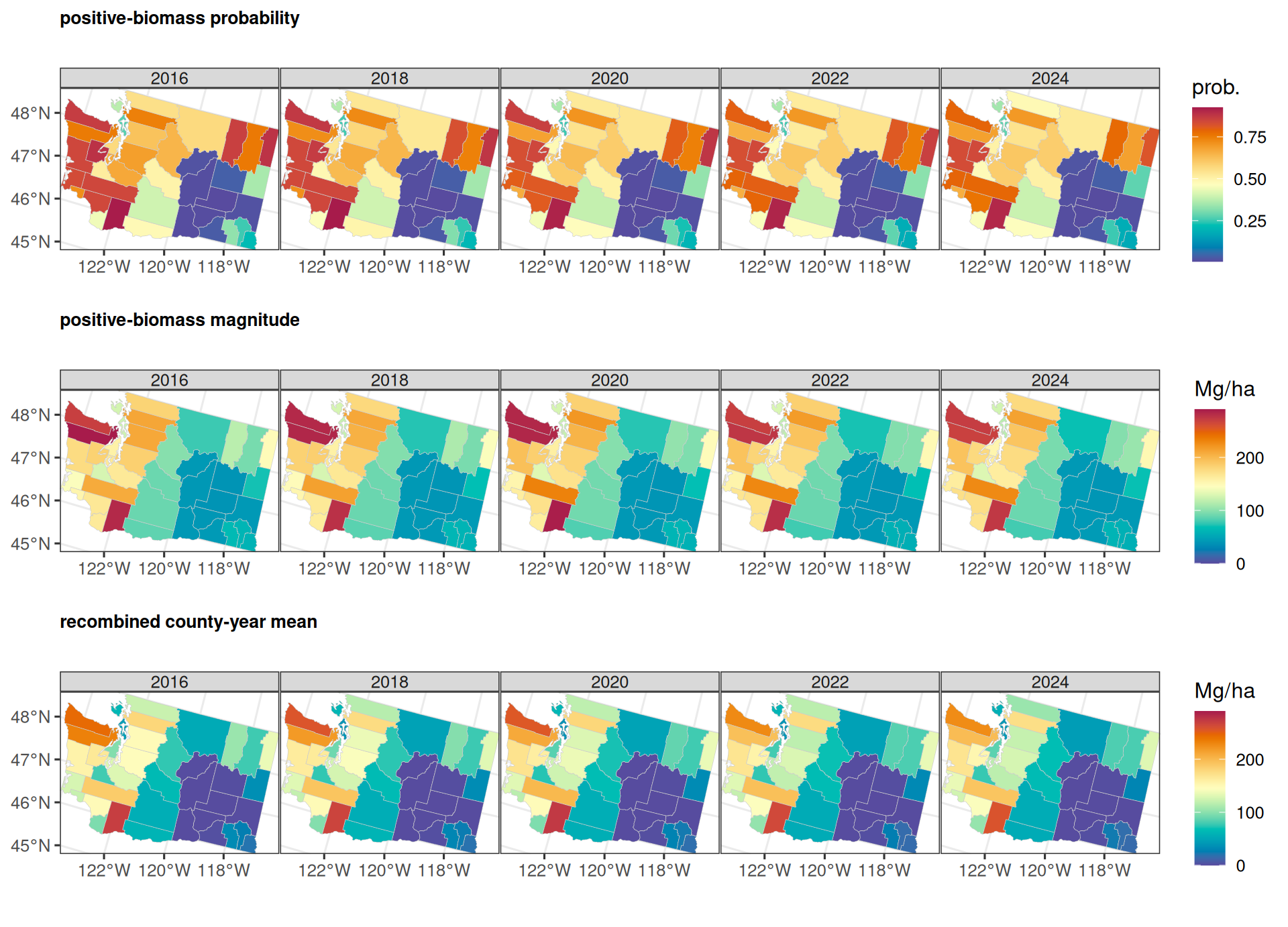
The maps separate the two model stages before showing the recombined series target. The first row is the average positive-biomass probability, the second row is the positive-biomass magnitude from the Gaussian stage, and the third row is the recombined county-year mean. The two Mg/ha rows use the same color scale, anchored by the positive-biomass magnitude, so the recombined mean can be read as a damped product of occurrence and positive magnitude.
Show prediction map code
panel_years <- c(2016, 2018, 2020, 2022, 2024)

map_dat <- wa_counties |>
  left_join(
    county_summary |> filter(year %in% panel_years),
    by = "county_fips"
  )

biomass_map_limits <- c(0, max(map_dat$positive_mean, na.rm = TRUE))

component_map <- function(fill_var, legend_title, title, limits = NULL) {
  ggplot(map_dat) +
    geom_sf(aes(fill = .data[[fill_var]]), color = "grey80", linewidth = 0.12) +
    coord_sf(expand = FALSE) +
    facet_wrap(~ year, nrow = 1) +
    scale_fill_gradientn(
      colors = stlmm_palette(),
      name = legend_title,
      limits = limits,
      na.value = "grey92"
    ) +
    labs(title = title) +
    theme(
      panel.spacing = grid::unit(0.03, "lines"),
      strip.text = element_text(margin = margin(1, 1, 1, 1)),
      plot.title = element_text(size = 10, face = "bold", margin = margin(0, 0, 2, 0)),
      plot.margin = margin(0, 0, 0, 0)
    )
}

component_map(
  "p_positive_mean",
  "prob.",
  "positive-biomass probability"
) /
  component_map(
    "positive_mean",
    "Mg/ha",
    "positive-biomass magnitude",
    limits = biomass_map_limits
  ) /
  component_map(
    "theta_mean",
    "Mg/ha",
    "recombined county-year mean",
    limits = biomass_map_limits
  )
8 County Time Series
The time-series figure uses the same four counties as the opening unit-response article. Direct estimates are shown where county-year direct estimates are model-ready.
Show county time-series code
profile_counties <- c("Clallam", "King", "Okanogan", "Yakima")

profile_dat <- county_summary |>
  filter(county %in% profile_counties) |>
  mutate(county = factor(county, levels = profile_counties))

ggplot(profile_dat, aes(year, theta_mean)) +
  geom_ribbon(
    aes(ymin = theta_lower, ymax = theta_upper),
    fill = stlmm_color("primary"),
    alpha = 0.15,
    color = NA
  ) +
  geom_line(color = stlmm_color("primary"), linewidth = 0.75) +
  geom_point(
    aes(y = direct_biomass_model),
    color = "grey20",
    size = 1.4,
    alpha = 0.75,
    na.rm = TRUE
  ) +
  facet_wrap(~ county, scales = "free_y", ncol = 2) +
  labs(
    x = "year",
    y = "mean agb_live_mg_ha (Mg/ha)"
  )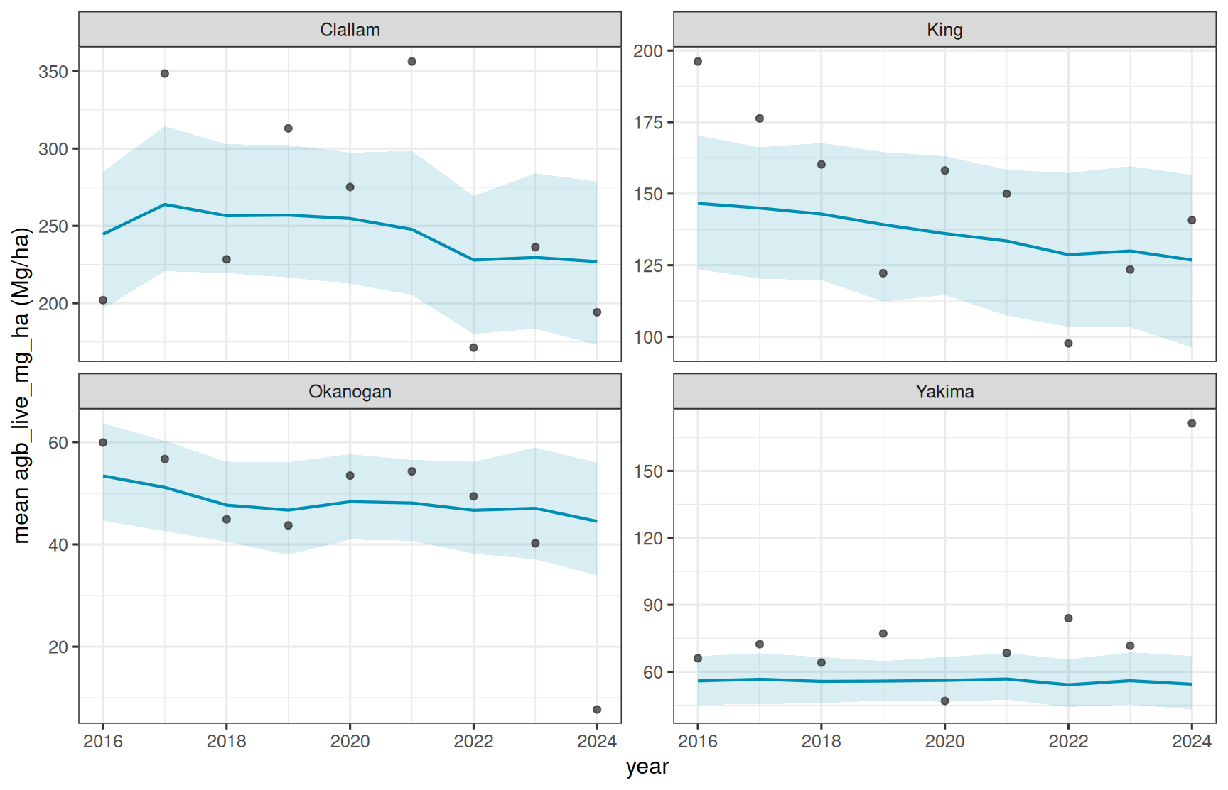
As in the previous BHF analysis, the Yakima predictions are consistently below many of the direct estimates. Importantly, the direct estimates are not the target for these models; we include them to show where the unit-response summaries agree with the direct estimates and where they differ. Yakima is useful for seeing the difference between fitting the observed plot rows and aggregating over a prediction support. In the data used here, Yakima’s observed plot rows have higher mean TCC than the prediction grid. Averaged over the modeled years, the observed Yakima plot rows have mean TCC about 31, while the 5 km prediction grid has mean TCC about 25. Because TCC is positively related to both positive-biomass occurrence and positive-biomass magnitude, applying the model over the lower-TCC grid support shifts the county-year prediction downward.
This is not a failure of the fitted model. If the biomass-TCC relationship is estimated well and the grid is the intended support, the unit-response model may be compensating for a sampled plot support that is not representative of the county-wide TCC distribution. The important caveats are that this interpretation depends on the model: TCC must be an adequate adjustment variable, the fitted relationship must transport from sampled plots to grid cells, and the grid must represent the target support we intend to estimate. Under those assumptions, disagreement with the simple direct estimate can be a useful feature of the unit-response approach rather than a symptom that the model missed Yakima.
9 Takeaways
This model is the first structured unit-response analogue of the area-response CAR-time plus TCC articles. It keeps the same series target, uses agb_live_mg_ha > 0 for the two-stage split, and adds a county-year process so counties can have their own temporal patterns.
The next unit-response article can keep this same two-stage CAR-time TCC mean structure and add FIA-unit-specific residual variance in the positive Gaussian stage. The binary stage has no Gaussian residual variance term, so the heteroskedastic extension belongs only in the positive-biomass stage.