
Unit-response two-stage continuous space-time model with spatial SVC
Washington biomass prediction with row-level TCC, FIA-unit variances, and a positive-stage spatial SVC
Source:vignettes/wa-unit-two-stage-continuous-space-time-tcc-fiaunit-var-svc.qmd
1 Purpose
This article carries forward the two-stage unit-response target used in the previous articles and changes the latent process. The binary stage still models agb_live_mg_ha > 0, the positive stage still models square-root positive agb_live_mg_ha, row-level TCC remains the auxiliary covariate, and the county-year target remains the grid-supported mean of agb_live_mg_ha.
The new feature is the space-time process. The earlier unit-response articles used county-year areal effects, first through simple county and year effects and then through car_time(county_fips, year). Here, the latent process is indexed by continuous projected coordinates and measurement time.
A continuous space-time process also makes prediction less tied to the administrative units used for fitting. Once the model is fit, predictions can be made on any user-defined spatial extent or grid with the required covariates, then summarized over counties, ownerships, ecological regions, management areas, or other supports. This is a central advantage of the unit-response space-time approach used in related forest-biomass applications (Finley et al. 2011; May and Finley 2025).
The positive Gaussian stage carries forward the FIA-unit-specific residual variance from the previous article. That variance refinement is paired here with a positive-stage spatially varying coefficient (SVC), so the TCC-biomass relationship can change smoothly over space rather than being forced to use one global positive-biomass slope.
The fitted model is intentionally rich. It combines a two-stage response, continuous space-time NNGP intercept processes, FIA-unit-specific residual variances, and a spatially varying TCC effect in the positive biomass stage. Before using this kind of model for a final analysis, check that the data identify the added parameters and compare predictive performance using WAIC or, preferably, a cross-validation study.
For plot row \(j\) with coordinates \(\mathbf{s}_j\), measurement time \(t_j\), county \(a_j\), FIA unit \(u_j\), and standardized TCC \(x_j\), the model is
\[ z_j \sim \operatorname{bernoulli}(p_j), \qquad \operatorname{logit}(p_j) = \gamma_0 + \gamma_1 x_j + w^z(\mathbf{s}_j, t_j), \]
and, for positive biomass rows,
\[ q_j = \delta_0 + \{\delta_1 + v^+(\mathbf{s}_j)\}x_j + w^+(\mathbf{s}_j, t_j) + r_j,\qquad r_j \sim \operatorname{normal}(0,\tau^2_{u_j}), \]
where \(z_j = \mathbb{1}(y_j > 0)\) and \(q_j = \sqrt{y_j^+}\). The processes \(w^z(\mathbf{s}_j, t_j)\) and \(w^+(\mathbf{s}_j, t_j)\) are occurrence-stage and positive-stage space-time intercept surfaces, respectively, and \(v^+(\mathbf{s}_j)\) is the spatial departure from the global positive-stage TCC slope. Prediction combines draw-matched binary and positive-stage draws on grid row \(g\),
\[ \tilde{y}^{(m)}_g = \tilde{z}^{(m)}_g\{\tilde{q}^{(m)}_g\}^2, \]
then averages over grid rows within county-year.
2 Data
Show data-reading code
wa_counties <- read_rds(file.path(data_dir, "wa_counties.rds"))
unit_plots <- read_csv(file.path(data_dir, "wa_unit_plots.csv"), show_col_types = FALSE)
direct_estimates <- read_csv(file.path(data_dir, "wa_direct_estimates.csv"), show_col_types = FALSE)
prediction_grid <- read_csv(
  file.path(data_dir, "wa_unit_prediction_grid_5km.csv"),
  show_col_types = FALSE
)

wa_counties <- wa_counties |>
  mutate(
    county_fips = as.character(county_fips),
    fia_unit = factor(fia_unit)
  )

unit_plots <- unit_plots |>
  mutate(
    county_fips = as.character(county_fips),
    county_fips = factor(county_fips),
    fia_unit = factor(fia_unit),
    year = as.integer(year),
    time = as.numeric(time),
    x_km = x / 1000,
    y_km = y / 1000,
    biomass_positive = as.integer(agb_live_mg_ha > 0)
  ) |>
  arrange(county_fips, year, plot_id)

direct_estimates <- direct_estimates |>
  mutate(
    county_fips = as.character(county_fips),
    year = as.integer(year)
  )

plot_years <- sort(unique(unit_plots$year))
tcc_center <- mean(unit_plots$tcc_mean, na.rm = TRUE)
tcc_scale <- sd(unit_plots$tcc_mean, na.rm = TRUE)

unit_plots <- unit_plots |>
  mutate(tcc_mean_scaled = (tcc_mean - tcc_center) / tcc_scale)

county_levels <- levels(unit_plots$county_fips)
fia_unit_levels <- levels(unit_plots$fia_unit)
fia_unit_names <- unit_plots |>
  distinct(fia_unit, fia_unit_name) |>
  arrange(fia_unit)

prediction_grid <- prediction_grid |>
  mutate(
    county_fips = as.character(county_fips),
    county_fips = factor(county_fips, levels = county_levels),
    fia_unit = factor(fia_unit, levels = fia_unit_levels),
    year = as.integer(year),
    time = as.numeric(year),
    tcc_mean_scaled = (tcc_mean - tcc_center) / tcc_scale
  ) |>
  filter(year %in% plot_years) |>
  arrange(county_fips, year, x, y)

positive_plots <- unit_plots |>
  filter(biomass_positive == 1) |>
  mutate(biomass_sqrt = sqrt(agb_live_mg_ha))
The plot rows include time, a decimal measurement year used by the continuous space-time process. The prediction grid is annual, so its prediction time is set to the integer year for the county-year support being summarized. Plot-level and grid-level TCC values are annual point samples from the USDA Forest Service Tree Canopy Cover raster products (USDA Forest Service 2026). The model uses the same plot-based TCC standardization for plot rows and prediction-grid rows.
Show data summary code
data_summary <- tibble(
  quantity = c(
    "plot rows",
    "positive-biomass plot rows",
    "FIA units",
    "5 km prediction-grid rows",
    "measurement years"
  ),
  value = c(
    fmt_int(nrow(unit_plots)),
    fmt_int(nrow(positive_plots)),
    fmt_int(n_distinct(unit_plots$fia_unit)),
    fmt_int(nrow(prediction_grid)),
    paste(range(plot_years), collapse = "-")
  )
)

show_table(data_summary, caption = "Unit-response data for the continuous space-time model with spatial SVC.")| quantity | value |
|---|---|
| plot rows | 6,935 |
| positive-biomass plot rows | 3,991 |
| FIA units | 5 |
| 5 km prediction-grid rows | 63,306 |
| measurement years | 2016-2024 |
Show plot map code
ggplot() +
  geom_sf(data = wa_counties, fill = "grey96", color = "grey70", linewidth = 0.2) +
  geom_point(
    data = unit_plots,
    aes(x, y, color = time),
    size = 0.35,
    alpha = 0.55
  ) +
  coord_sf(expand = FALSE) +
  scale_color_gradientn(colors = stlmm_palette(), name = "measurement time") +
  labs(x = NULL, y = NULL)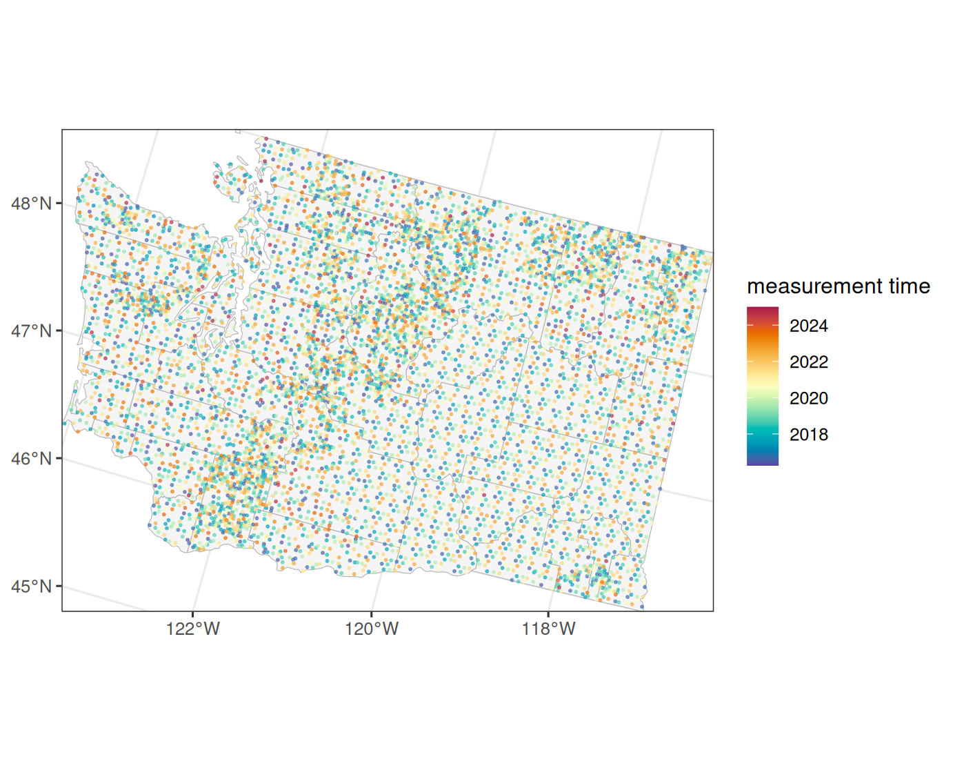
3 Model Settings
The occurrence and positive-biomass intercept processes use multi_res_sep_exp, the two-scale separable exponential space-time covariance proposed by May and Finley (2025). The covariance is a weighted sum of broad and local separable exponential components. The broad component represents large-scale, slowly varying space-time structure, while the local component represents shorter-range departures. Coordinates are modeled in kilometers and time is modeled in years so the spatial and temporal decay parameters have direct range interpretations.
The positive-stage TCC SVC uses a simpler spatial exponential NNGP. That reflects the working assumption that the positive-biomass relationship with TCC can differ among regions but is not expected to change materially over the measurement period.
stLMM parameterizes exponential correlations as exp(-phi * distance). If range_05 is the distance where correlation reaches 0.05, then phi = -log(0.05) / range_05. The broad component uses lower spatial decay and the local component uses higher spatial decay through non-overlapping prior ranges.
In the model settings below, chains are kept intentionally short so the vignette renders quickly. Longer runs with at least 15,000 MCMC samples per chain produced satisfactory convergence diagnostics for all model parameters. The starting values below are based on those longer runs. For an actual analysis, use dispersed starting values and longer runs, with appropriate warmup and convergence checks.
Show model settings code
cor_at_range <- 0.05

decay_from_range <- function(range_05) {
  -log(cor_at_range) / range_05
}

## Broad process: approximately 25-100 km and 1-500 years.
phi_1_bounds <- decay_from_range(rev(c(25, 100)))
lambda_1_bounds <- decay_from_range(rev(c(1, 500)))

## Local process: approximately 1-25 km and 1-500 years.
phi_2_bounds <- decay_from_range(rev(c(1, 25)))
lambda_2_bounds <- decay_from_range(rev(c(1, 500)))

## Spatial SVC process: approximately 10-150 km.
phi_svc_bounds <- decay_from_range(rev(c(10, 150)))

n_samples <- 1000
burnin <- 1
chains <- 3
n_keep <- 25
posterior_thin <- max(1L, floor((n_samples - burnin) / n_keep))
posterior_sub_sample <- list(start = burnin + 1, thin = posterior_thin)
n_report <- 500

## Let stLMM use OpenMP threads while preventing BLAS from nesting threads
## inside the sampler and prediction calculations.
blas_set_num_threads(1)
n_omp_threads <- as.integer(Sys.getenv("STLMM_OMP_THREADS", unset = "25"))

fit_st_scale <- 2
pred_st_scale <- fit_st_scale

sqrt_response_sd <- sd(positive_plots$biomass_sqrt, na.rm = TRUE)
The st_scale value affects NNGP ordering and neighbor search, not the covariance function itself. Here, one year of separation is treated like about two kilometers for ordering and neighbor search. The covariance still evaluates spatial distance in kilometers and temporal distance in years.
Show starting value code
jitter_start <- function(value, amount = 0.01, bounds = NULL) {
  out <- rep(value, chains) * exp(rnorm(chains, 0, amount))

  if (!is.null(bounds)) {
    out <- pmin(pmax(out, bounds[1] + 1e-8), bounds[2] - 1e-8)
  }

  out
}


occurrence_start <- list(
  beta = c(
    `(Intercept)` = -0.18,
    tcc_mean_scaled = 10
  ),
  nngp_1 = list(
    sigma_sq = 80,
    alpha = 0.52,
    phi_1 = 0.031,
    lambda_1 = 0.039,
    phi_2 = 1.7,
    lambda_2 = 1.6
  )
)

biomass_start <- list(
  resid = list(
    tau_sq = c(
      `5` = 28,
      `6` = 25,
      `7` = 26,
      `8` = 12,
      `9` = 11
    )
  ),
  nngp_1 = list(
    sigma_sq = 2.3,
    alpha = 0.74,
    phi_1 = 0.037,
    lambda_1 = 0.059,
    phi_2 = 1.6,
    lambda_2 = 1.5
  ),
  nngp_2 = list(
    sigma_sq = 2.4,
    phi = 0.027
  )
)

occurrence_starting <- list(
  beta = occurrence_start$beta,
  nngp_1 = list(
    sigma_sq = jitter_start(occurrence_start$nngp_1$sigma_sq),
    alpha = jitter_start(occurrence_start$nngp_1$alpha, bounds = c(0, 1)),
    phi_1 = jitter_start(occurrence_start$nngp_1$phi_1, bounds = phi_1_bounds),
    lambda_1 = jitter_start(occurrence_start$nngp_1$lambda_1, bounds = lambda_1_bounds),
    phi_2 = jitter_start(occurrence_start$nngp_1$phi_2, bounds = phi_2_bounds),
    lambda_2 = jitter_start(occurrence_start$nngp_1$lambda_2, bounds = lambda_2_bounds)
  )
)

biomass_starting <- list(
  resid = biomass_start$resid,
  nngp_1 = list(
    sigma_sq = jitter_start(biomass_start$nngp_1$sigma_sq),
    alpha = jitter_start(biomass_start$nngp_1$alpha, bounds = c(0, 1)),
    phi_1 = jitter_start(biomass_start$nngp_1$phi_1, bounds = phi_1_bounds),
    lambda_1 = jitter_start(biomass_start$nngp_1$lambda_1, bounds = lambda_1_bounds),
    phi_2 = jitter_start(biomass_start$nngp_1$phi_2, bounds = phi_2_bounds),
    lambda_2 = jitter_start(biomass_start$nngp_1$lambda_2, bounds = lambda_2_bounds)
  ),
  nngp_2 = list(
    sigma_sq = jitter_start(biomass_start$nngp_2$sigma_sq),
    phi = jitter_start(biomass_start$nngp_2$phi, bounds = phi_svc_bounds)
  )
)
4 Fit
The binary model uses all plot rows and models whether agb_live_mg_ha is positive.
occurrence_fit <- stLMM(
  biomass_positive ~
    tcc_mean_scaled +
    nngp(x_km, y_km, time,
         m = 15,
         cov_model = "multi_res_sep_exp",
         ordering = "maxmin",
         st_scale = fit_st_scale),
  data = unit_plots,
  family = "binomial",
  starting = occurrence_starting,
  priors = list(
    beta = normal(mean = 0, sd = 2.5),
    nngp_1 = list(
      sigma_sq = log_normal(meanlog = log(100), sdlog = 0.15),
      alpha = uniform(0, 1),
      phi_1 = uniform(phi_1_bounds[1], phi_1_bounds[2]),
      lambda_1 = uniform(lambda_1_bounds[1], lambda_1_bounds[2]),
      phi_2 = uniform(phi_2_bounds[1], phi_2_bounds[2]),
      lambda_2 = uniform(lambda_2_bounds[1], lambda_2_bounds[2])
    )
  ),
  n_samples = n_samples,
  chains = chains,
  save_process = posterior_sub_sample,
  n_omp_threads = n_omp_threads,
  verbose = TRUE,
  n_report = n_report
)
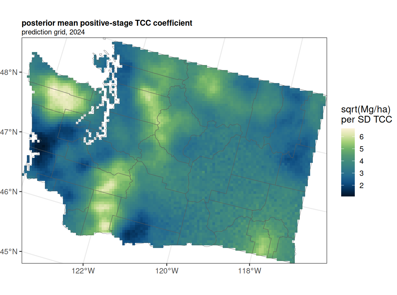
The positive stage models square-root positive biomass, carries forward FIA-unit-specific residual variances, and adds a positive-stage spatial TCC SVC. The term tcc_mean_scaled:nngp(x_km, y_km, ...) is a spatial process multiplied by the standardized TCC value, so it represents regional departures from the global positive-biomass TCC slope.
biomass_fit <- stLMM(
  biomass_sqrt ~
    tcc_mean_scaled +
    nngp(x_km, y_km, time,
         m = 15,
         cov_model = "multi_res_sep_exp",
         ordering = "maxmin",
         st_scale = fit_st_scale) +
    tcc_mean_scaled:nngp(x_km, y_km,
         m = 15,
         cov_model = "exp",
         ordering = "maxmin") +
    resid(model = "group", group = fia_unit),
  data = positive_plots,
  starting = biomass_starting,
  priors = list(
    beta = normal(mean = 0, sd = 2 * sqrt_response_sd),
    resid = list(tau_sq = half_t(df = 3, scale = sqrt_response_sd)),
    nngp_1 = list(
      sigma_sq = half_t(df = 3, scale = sqrt_response_sd),
      alpha = uniform(0, 1),
      phi_1 = uniform(phi_1_bounds[1], phi_1_bounds[2]),
      lambda_1 = uniform(lambda_1_bounds[1], lambda_1_bounds[2]),
      phi_2 = uniform(phi_2_bounds[1], phi_2_bounds[2]),
      lambda_2 = uniform(lambda_2_bounds[1], lambda_2_bounds[2])
    ),
    nngp_2 = list(
      sigma_sq = half_t(df = 3, scale = 0.5 * sqrt_response_sd),
      phi = uniform(phi_svc_bounds[1], phi_svc_bounds[2])
    )
  ),
  n_samples = n_samples,
  chains = chains,
  n_omp_threads = n_omp_threads,
  verbose = TRUE,
  n_report = n_report
)
Show fit summaries
occurrence_summary$parameters mean sd q2.5 q50.0 q97.5
(Intercept) -0.17055020 0.882000281 -1.914944668 -0.18556097 1.57967114
tcc_mean_scaled 9.97743523 0.729200872 8.733449938 9.89474529 11.70783308
nngp_1_sigma_sq 71.12837827 9.252177112 56.289621707 69.75632869 93.07003511
nngp_1_alpha 0.52992684 0.041377140 0.447766600 0.52827890 0.60576509
nngp_1_phi_1 0.03134155 0.001178761 0.030031384 0.03099035 0.03456605
nngp_1_lambda_1 0.03236267 0.015633883 0.007458989 0.03055200 0.06561046
nngp_1_phi_2 1.58063559 0.539949956 0.546795700 1.62226334 2.53350014
nngp_1_lambda_2 1.66649602 0.521713654 0.614287012 1.67943371 2.73000616Show fit summaries
biomass_summary$parameters mean sd q2.5 q50.0 q97.5
(Intercept) 9.54918956 0.246692937 9.08310735 9.54364644 10.05411771
tcc_mean_scaled 3.62081888 0.356951667 2.90709046 3.62419376 4.36743932
tau_sq_9 11.84230557 0.724981234 10.39456006 11.86705530 13.19913858
tau_sq_8 12.29822863 0.648828682 10.86757417 12.28929358 13.54536036
tau_sq_6 25.87493631 1.780531575 22.36287940 25.78260202 29.37465666
tau_sq_7 26.14674794 1.461023582 23.47157442 26.13997757 28.96430282
tau_sq_5 28.29600766 1.609589200 25.26230040 28.24182688 31.68922943
nngp_1_sigma_sq 2.35952160 0.549300942 1.34889812 2.32130432 3.61902163
nngp_2_sigma_sq 2.29800898 0.612406953 1.19645012 2.27327011 3.62914340
nngp_1_alpha 0.74743325 0.086115895 0.53867702 0.76325790 0.86367456
nngp_1_phi_1 0.03595209 0.004233696 0.03106535 0.03483039 0.04701873
nngp_1_lambda_1 0.05860021 0.022332765 0.02313445 0.05768881 0.10647616
nngp_1_phi_2 1.60795735 0.232620835 1.10678198 1.62256793 2.01399166
nngp_1_lambda_2 1.50377836 0.462077198 0.74134724 1.46819562 2.75140240
nngp_2_phi 0.02856079 0.005194730 0.02287582 0.02691175 0.04341740The tcc_mean_scaled row in the positive-stage summary is the global TCC slope on the square-root positive-biomass scale. The nngp_2 rows describe the spatial process that modifies that slope. Thus, at a given location, the positive-stage TCC coefficient is the global slope plus the local draw from the SVC process. This SVC is used only in the positive biomass stage; the occurrence stage keeps a single global TCC slope.
5 Fitted Space-Time Ranges
The table below reports posterior median practical ranges, defined as the spatial or temporal lag where correlation is approximately 0.05. The positive-stage SVC has its own spatial covariance parameter because it is a second NNGP process.
Show fitted covariance summary code
posterior_medians <- function(fit) {
  draws <- as_samples(fit, burn = burnin, metadata = FALSE)
  apply(draws, 2, stats::median)
}

param_value <- function(x, name) {
  unname(x[name])
}

occurrence_medians <- posterior_medians(occurrence_fit)
biomass_medians <- posterior_medians(biomass_fit)

practical_ranges <- function(p, model, process) {
  tibble(
    model = model,
    component = c("broad", "local"),
    spatial_range_km = -log(cor_at_range) / c(
      param_value(p, paste0(process, "_phi_1")),
      param_value(p, paste0(process, "_phi_2"))
    ),
    temporal_range_years = -log(cor_at_range) / c(
      param_value(p, paste0(process, "_lambda_1")),
      param_value(p, paste0(process, "_lambda_2"))
    ),
    variance_weight = c(
      param_value(p, paste0(process, "_alpha")),
      1 - param_value(p, paste0(process, "_alpha"))
    )
  )
}

range_summary <- bind_rows(
  practical_ranges(occurrence_medians, "positive-biomass occurrence", "nngp_1"),
  practical_ranges(biomass_medians, "sqrt positive biomass intercept", "nngp_1"),
  tibble(
    model = "sqrt positive biomass TCC SVC",
    component = "spatial",
    spatial_range_km = -log(cor_at_range) / param_value(biomass_medians, "nngp_2_phi"),
    temporal_range_years = NA_real_,
    variance_weight = NA_real_
  )
) |>
  mutate(across(where(is.numeric), ~ round(.x, 2)))

show_table(
  range_summary,
  caption = "Posterior median practical ranges for the intercept and spatial SVC covariance components."
)| model | component | spatial_range_km | temporal_range_years | variance_weight |
|---|---|---|---|---|
| positive-biomass occurrence | broad | 96.67 | 98.05 | 0.53 |
| positive-biomass occurrence | local | 1.85 | 1.78 | 0.47 |
| sqrt positive biomass intercept | broad | 86.01 | 51.93 | 0.76 |
| sqrt positive biomass intercept | local | 1.85 | 2.04 | 0.24 |
| sqrt positive biomass TCC SVC | spatial | 111.32 | NA | NA |
Show FIA-unit residual SD table code
biomass_draws <- as_samples(biomass_fit, burn = burnin, metadata = FALSE)
resid_var_names <- paste0("tau_sq_", fia_unit_levels)
if (!all(resid_var_names %in% colnames(biomass_draws))) {
  resid_var_names <- fia_unit_levels
}
resid_sd_draws <- sqrt(biomass_draws[, resid_var_names, drop = FALSE])

fia_resid_sd <- tibble(
  fia_unit = factor(fia_unit_levels, levels = fia_unit_levels),
  sd_mean = colMeans(resid_sd_draws),
  sd_lower = apply(resid_sd_draws, 2, quantile, probs = 0.025),
  sd_upper = apply(resid_sd_draws, 2, quantile, probs = 0.975)
) |>
  left_join(fia_unit_names, by = "fia_unit")

show_table(
  fia_resid_sd |>
    transmute(
      `FIA unit` = fia_unit_name,
      `posterior mean SD` = fmt_num(sd_mean, 2),
      `lower` = fmt_num(sd_lower, 2),
      `upper` = fmt_num(sd_upper, 2)
    ),
  caption = "FIA-unit residual standard deviations for square-root positive biomass."
)| FIA unit | posterior mean SD | lower | upper |
|---|---|---|---|
| Puget Sound | 5.32 | 5.03 | 5.63 |
| Olympic Peninsula | 5.08 | 4.73 | 5.42 |
| Southwest | 5.11 | 4.84 | 5.38 |
| Central | 3.51 | 3.30 | 3.68 |
| Inland Empire | 3.44 | 3.22 | 3.63 |
6 Prediction and Aggregation
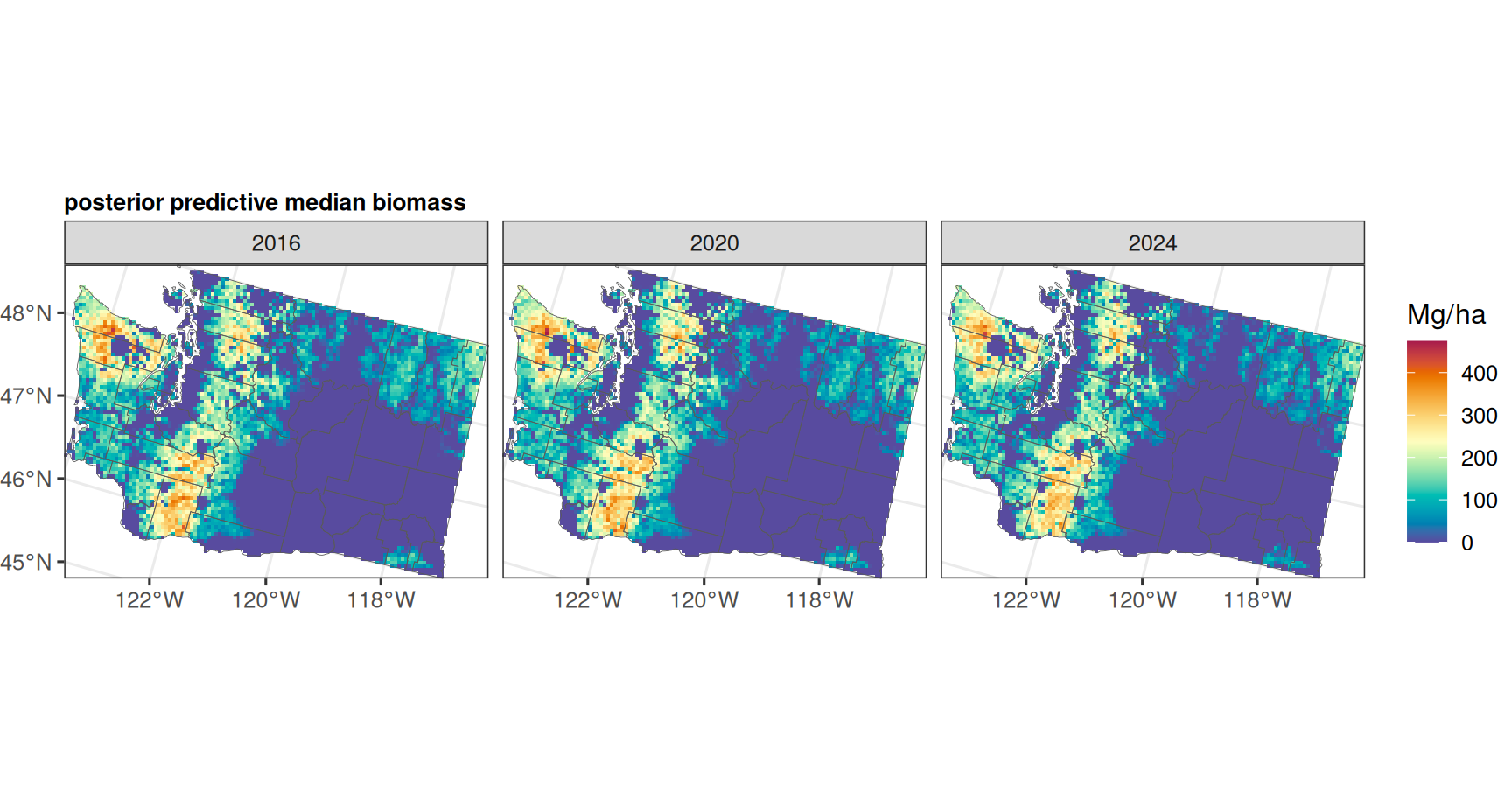
The model predicts at all annual 5 km grid rows. For the full grid aggregation, this article uses independent NNGP prediction for computational tractability. Joint Vecchia prediction is the heavier alternative when the primary focus is aggregate posterior uncertainty over a dense prediction lattice. The Gaussian positive-stage predictions use posterior predictive draws on the square-root scale before squaring, so the recombined biomass draws include positive-stage residual uncertainty. A separate one-year prediction keeps draws of the positive-stage SVC process so the grid-level TCC coefficient can be summarized without storing process draws for every annual grid row.
Show aggregation helper code
prediction_sample_matrix <- function(pred, sample, include_w = FALSE) {
  as.matrix(as_samples(
    pred,
    sample = sample,
    include_w = include_w,
    metadata = FALSE
  ))
}

prediction_w_matrix <- function(pred, term) {
  draws <- prediction_sample_matrix(pred, "mu", include_w = TRUE)
  w_cols <- grep(paste0("^w_", term, "_"), colnames(draws), value = TRUE)

  if (!length(w_cols)) {
    stop("No predicted process samples found for ", term, call. = FALSE)
  }

  draws[, w_cols, drop = FALSE]
}

aggregate_grid_draws <- function(draws, grid, prefix = "") {
  county_year <- grid |>
    distinct(county_fips, county, year) |>
    arrange(county_fips, year)

  county_samples <- matrix(
    NA_real_,
    nrow = nrow(draws),
    ncol = nrow(county_year)
  )

  for (j in seq_len(nrow(county_year))) {
    ii <- which(
      grid$county_fips == county_year$county_fips[j] &
        grid$year == county_year$year[j]
    )
    county_samples[, j] <- rowMeans(draws[, ii, drop = FALSE])
  }

  county_year |>
    bind_cols(
      summarize_draw_matrix(county_samples, prefix = prefix) |>
        select(-prediction_row)
    )
}
occurrence_pred <- predict(
  occurrence_rec,
  newdata = prediction_grid,
  y_samples = TRUE,
  st_scale = pred_st_scale,
  return_w_samples = FALSE
)

biomass_pred <- predict(
  biomass_rec,
  newdata = prediction_grid,
  y_samples = TRUE,
  return_w_samples = FALSE
)

svc_map_year <- 2024
svc_prediction_grid <- prediction_grid |>
  filter(year == svc_map_year)

biomass_svc_pred <- predict(
  biomass_rec,
  newdata = svc_prediction_grid,
  y_samples = FALSE,
  return_w_samples = TRUE
)
Show direct-estimate join code
direct_for_compare <- direct_estimates |>
  filter(year %in% plot_years) |>
  select(
    county_fips, county, year, n,
    direct_biomass_model, direct_biomass_se_model
  )

county_summary <- county_summary |>
  mutate(county_fips = as.character(county_fips)) |>
  left_join(
    direct_for_compare,
    by = c("county_fips", "county", "year")
  )
Show prediction map code
ggplot() +
  geom_raster(
    data = prediction_map,
    aes(x, y, fill = theta_median)
  ) +
  geom_sf(data = wa_counties, fill = NA, color = "grey35", linewidth = 0.15) +
  facet_wrap(~ year, nrow = 1) +
  coord_sf(expand = FALSE) +
  scale_fill_gradientn(
    colors = stlmm_palette(),
    name = "Mg/ha",
    na.value = "grey92"
  ) +
  labs(
    title = "posterior predictive median biomass",
    x = NULL,
    y = NULL
  ) +
  theme(
    plot.title = element_text(size = 10, face = "bold", margin = margin(0, 0, 2, 0)),
    plot.margin = margin(0, 0, 0, 0)
  )
The SVC term can also be viewed directly on the prediction grid. The map below summarizes the positive-stage TCC coefficient, which is the global tcc_mean_scaled slope plus the predicted local SVC draw. The coefficient is on the square-root positive-biomass scale and is measured per one standard deviation increase in TCC. Because this SVC is spatial-only, the coefficient surface does not change by year; the displayed year is just the grid slice used for mapping.
Show TCC SVC grid map code
ggplot() +
  geom_raster(
    data = tcc_coef_map,
    aes(x, y, fill = tcc_coef_mean)
  ) +
  geom_sf(data = wa_counties, fill = NA, color = "grey35", linewidth = 0.15) +
  coord_sf(expand = FALSE) +
  scale_fill_gradientn(
    colors = stlmm_continuous_palette(palette = "navia"),
    name = "sqrt(Mg/ha)\nper SD TCC",
    na.value = "grey92"
  ) +
  labs(
    title = "posterior mean positive-stage TCC coefficient",
    subtitle = paste("prediction grid,", svc_map_year),
    x = NULL,
    y = NULL
  ) +
  theme(
    plot.title = element_text(size = 10, face = "bold", margin = margin(0, 0, 2, 0)),
    plot.subtitle = element_text(size = 9, margin = margin(0, 0, 2, 0)),
    plot.margin = margin(0, 0, 0, 0)
  )
Show selected county-year summary code
show_table(
  county_summary |>
    filter(year == 2024) |>
    arrange(desc(theta_mean)) |>
    select(county, n, direct_biomass_model, theta_mean, theta_lower, theta_upper) |>
    slice_head(n = 10) |>
    mutate(
      across(
        c(direct_biomass_model, theta_mean, theta_lower, theta_upper),
        ~ fmt_num(.x, 1)
      )
    ),
  caption = "Highest 2024 county-year posterior predictive means from the continuous space-time model with spatial SVC."
)| county | n | direct_biomass_model | theta_mean | theta_lower | theta_upper |
|---|---|---|---|---|---|
| Skamania | 0 | NA | 264.0 | 235.7 | 292.2 |
| Clallam | 3 | 194.2 | 230.0 | 199.6 | 266.3 |
| Jefferson | 2 | 139.0 | 204.8 | 167.7 | 235.3 |
| Lewis | 3 | 80.3 | 185.8 | 165.6 | 212.3 |
| Skagit | 5 | 183.8 | 160.4 | 138.2 | 182.2 |
| Grays Harbor | 3 | 145.9 | 158.6 | 139.3 | 179.9 |
| Mason | 1 | NA | 157.4 | 127.2 | 191.1 |
| Cowlitz | 2 | 0.0 | 145.5 | 120.4 | 170.4 |
| Snohomish | 4 | 133.6 | 133.2 | 112.2 | 157.4 |
| King | 7 | 140.7 | 130.0 | 110.4 | 155.6 |
7 County Time Series
Show county time-series code
profile_counties <- c("Clallam", "King", "Okanogan", "Yakima")

profile_dat <- county_summary |>
  filter(county %in% profile_counties) |>
  mutate(county = factor(county, levels = profile_counties))

ggplot(profile_dat, aes(year, theta_mean)) +
  geom_ribbon(
    aes(ymin = theta_lower, ymax = theta_upper),
    fill = stlmm_color("primary"),
    alpha = 0.15,
    color = NA
  ) +
  geom_line(color = stlmm_color("primary"), linewidth = 0.75) +
  geom_point(
    aes(y = direct_biomass_model),
    color = "grey20",
    size = 1.4,
    alpha = 0.75,
    na.rm = TRUE
  ) +
  facet_wrap(~ county, scales = "free_y", ncol = 2) +
  labs(
    x = "year",
    y = "mean agb_live_mg_ha (Mg/ha)"
  )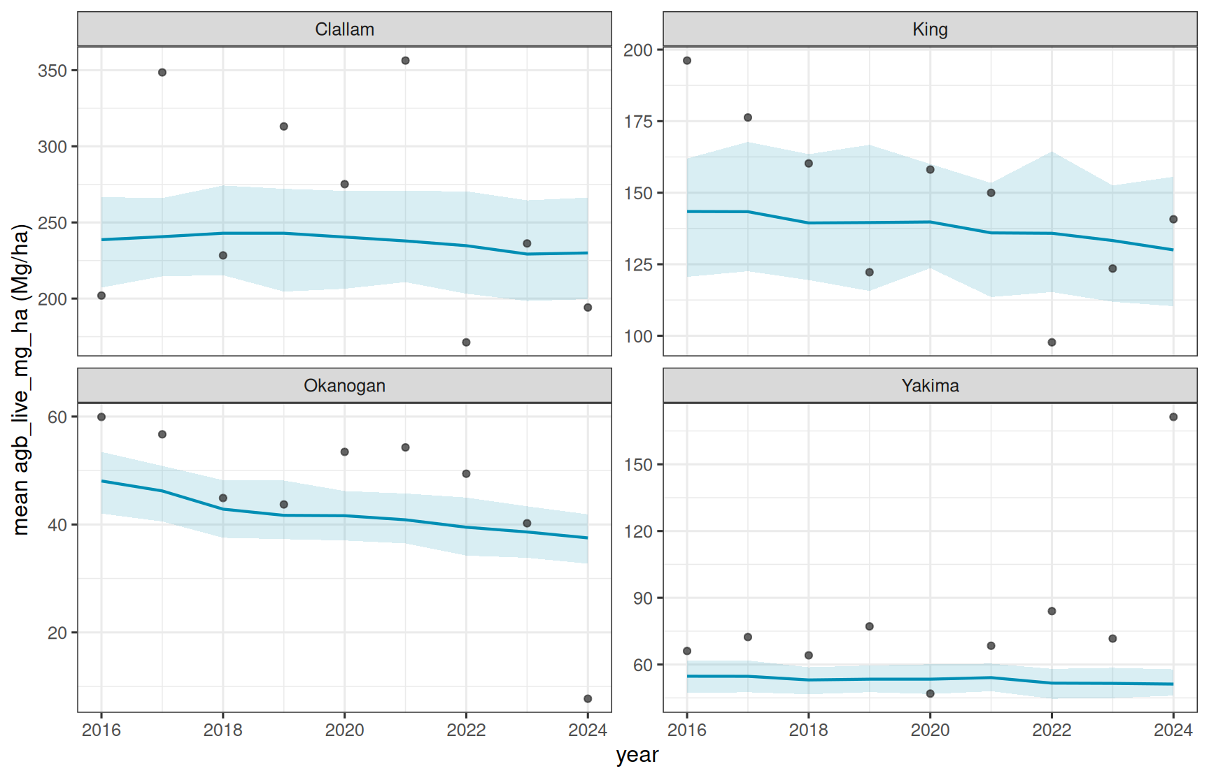
The direct estimates remain points of comparison rather than the model target. The main comparison with the previous unit-response articles is how the continuous space-time process changes the fitted county-year trajectories after prediction and aggregation over the same grid-supported response.
8 Takeaways
This article replaces county-year areal smoothing with continuous space-time NNGP intercept processes. The response definition, TCC covariate, two-stage product, FIA-unit residual variance in the positive stage, and county-year aggregation target are carried forward from the previous unit-response articles. The added SVC makes the positive-biomass TCC effect vary over continuous space.
The continuous process is useful when the model should borrow over distance and time without forcing all variation through county-year areal effects. The tradeoff is computational and inferential: dense grid prediction is more expensive than the areal CAR-time workflow, and the richer positive-stage mean model should be checked carefully before treating it as the preferred analysis model.