
Estimating Harvard Forest stand tables from sampled plots
Source:vignettes/articles/harvard-forest.qmd
This article examines how model structure affects species-by-DBH stand-table estimates and their uncertainty when only a small part of a forest is sampled. A mapped census of Harvard Forest provides known values for the forest and its four strata. We use sampled plots to fit the models and the census to assess their estimates.
We work through four steps:
- Fit models to one inventory. Starting with common intercepts, we add stratum and spatial effects in stages and compare fitted counts with observations.
- Assess prediction at held-out plots. Cross-validation shows how well each model predicts plots excluded from fitting.
- Estimate forest and stratum stand tables. We predict counts in unsampled areas, add the observed counts, and compare density estimates and intervals with the census.
- Repeat the sampling. Across 1,000 plot layouts in the same forest, we assess estimation error, interval coverage, and interval width. This shows whether conclusions from one inventory hold as the sampled locations change.
The species-by-DBH article introduces the model using simulated data. Here the population is a real forest, with features that our models may not fully describe. The aim is to understand what additional model structure contributes to the quantities we want to estimate, and where sparse observations still limit inference.
Example data and analysis
Download the Harvard Forest data (ZIP)
Extract the archive and use its harvard-forest folder as your R working directory. Use magComp 0.0.7 or later. The download includes the census, prepared inventory, sampling and fitting scripts, and result tables. The fitting code below can be run locally; the page uses saved summaries so it does not rerun the study when built.
Census and sampled plots
The 35-ha Harvard Forest CTFS–ForestGEO census contains mapped stem locations, species, and diameters, documented in the Harvard Forest Data Archive, HF253 (Orwig, Foster, and Ellison 2023). We use the processed first-census data accompanying Finley and Doser (2026); see the Harvard Forest data description. Our population contains 20,258 living stems with diameter at breast height (DBH) at least 12.7 cm.
We retain eastern hemlock, red maple, northern red oak, and eastern white pine separately, grouping the remaining species as Other. Six DBH classes give 30 species-by-DBH cells. Each class includes its lower endpoint and excludes its upper endpoint; 60+ includes all stems at least 60 cm DBH.
The four supplied strata are reporting areas that we also use to model differences in density and composition. Strata 1 and 4 are mixed conifer–hardwood forest, stratum 2 is conifer-dominated, and stratum 3 is a sparsely forested wetland, as described in the stratified-sampling example. We do not use environmental covariates in this study.
Sample the forest
We place circular plots of radius 9 m on a systematic grid with spacing about 88 m. A uniform random shift over one grid cell determines its position. The sampling frame extends 9 m beyond the forest boundary, allowing outside centers to sample trees inside the forest. This buffered-frame approach is illustrated in the Harvard Forest biomass example. The strata are not sampled separately.
Plots are clipped to the forest and split where they cross stratum boundaries. Each positive-area portion supplies its own counts and area, including portions with zero trees. All five models use these same observations. The first layout uses set.seed(1); the preparation code in sample_functions.R shows the random shift, clipping, and counting steps.
We begin by reading the polygons and satellite image, then show the strata, plot centers, and plot extents over the forest canopy.
Show plotting code
library(sf)
library(terra)
library(tidyterra)

forest <- st_read("inputs/forest.gpkg", quiet = TRUE)
strata <- st_read("inputs/strata.gpkg", quiet = TRUE)
centers <- st_read("data/plot_centers.gpkg", quiet = TRUE)
imagery <- rast("inputs/satellite.tif")
plot_extents <- st_buffer(centers, dist = 9)

ggplot() +
  geom_spatraster_rgb(data = imagery, r = 1, g = 2, b = 3) +
  geom_sf(data = strata, aes(fill = factor(stratum_id)), color = "white", alpha = 0.45) +
  geom_sf(data = plot_extents, fill = NA, color = "darkorange", linewidth = 0.5) +
  geom_sf(data = centers, color = "black", size = 0.7) +
  scale_fill_brewer(palette = "Pastel1", name = "Stratum") +
  guides(fill = guide_legend(override.aes = list(alpha = 1))) +
  coord_sf(datum = NA) +
  theme_void()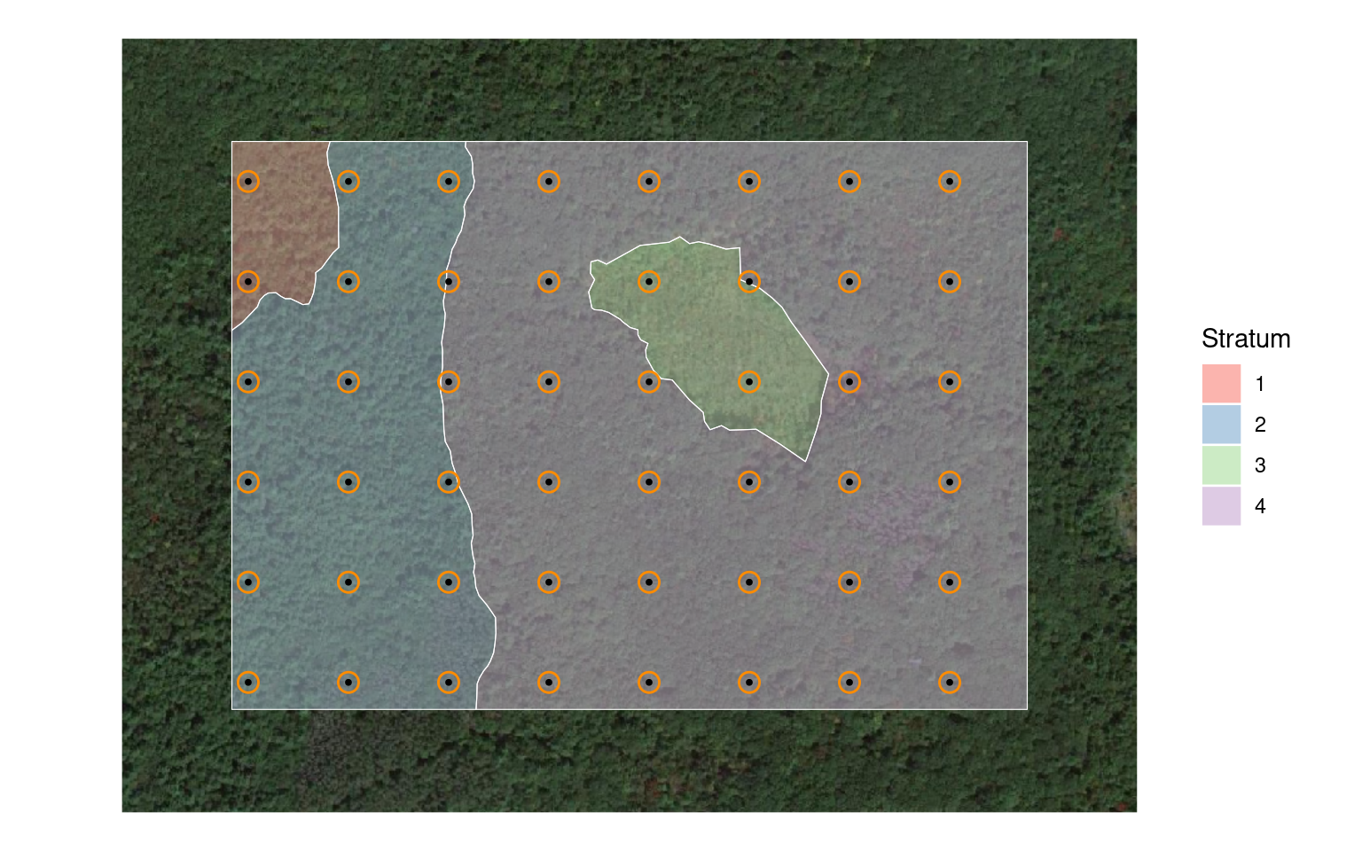
The 48 plots yield 52 stratum portions and 735 observed stems. plot_id identifies an original circle; unit_id identifies a portion used in fitting. Each portion has 30 rows, including empty species-by-DBH cells. For the spatial models, coordinates in kilometers locate the centroid of each sampled portion.
We read these counts and define the category order.
species_order <- c("Hemlock", "Red maple", "Red oak", "White pine", "Other")
dbh_classes <- c("12.7-20", "20-30", "30-40", "40-50", "50-60", "60+")

trees <- read_csv("data/ladder/trees.csv") |>
  mutate(species = factor(species, levels = species_order),
         dbh_class = ordered(dbh_class, levels = dbh_classes))

trees |>
  select(unit_id, plot_id, stratum_id, area_ha, species, dbh_class, count) |>
  head() |>
knitr::kable(digits = 4)| unit_id | plot_id | stratum_id | area_ha | species | dbh_class | count |
|---|---|---|---|---|---|---|
| 1 | 1 | 2 | 0.0254 | Hemlock | 12.7-20 | 1 |
| 1 | 1 | 2 | 0.0254 | Hemlock | 20-30 | 1 |
| 1 | 1 | 2 | 0.0254 | Hemlock | 30-40 | 4 |
| 1 | 1 | 2 | 0.0254 | Hemlock | 40-50 | 1 |
| 1 | 1 | 2 | 0.0254 | Hemlock | 50-60 | 0 |
| 1 | 1 | 2 | 0.0254 | Hemlock | 60+ | 1 |
The area summary shows how little information is available for some strata.
area_summary <- read_csv("data/area_summary.csv")

area_summary |>
  select(stratum_id, area_ha, plot_portions, sampled_area_ha, sampled_percent) |>
  knitr::kable(digits = 2, col.names = c(
    "Stratum", "Area (ha)", "Plot portions", "Sampled (ha)", "Sampled (%)"
))| Stratum | Area (ha) | Plot portions | Sampled (ha) | Sampled (%) |
|---|---|---|---|---|
| 1 | 1.24 | 2 | 0.05 | 4.12 |
| 2 | 8.93 | 16 | 0.37 | 4.10 |
| 3 | 2.25 | 3 | 0.06 | 2.70 |
| 4 | 22.58 | 31 | 0.74 | 3.29 |
Strata 1 and 3 have only two and three sampled portions, respectively. Their detailed stand tables will depend heavily on information shared across strata and on the model assumptions.
Add stratum and spatial effects in stages
Every model combines a negative-binomial total count with species allocation and DBH allocation within species. For portion , is expected stem density in trees per hectare, so its expected count is , where is the sampled area in hectares. The sequence below separates the contributions of stratum differences, within-species size distributions, and spatial dependence.
| Model | Magnitude | Species allocation | DBH allocation within species |
|---|---|---|---|
| H1 | Intercept | Intercepts | Intercepts |
| H2 | Intercept + stratum effect | Intercepts + stratum factor | Intercepts |
| H3 | As H2 | As H2 | Intercepts + stratum factor |
| H4 | As H3 + spatial effect | As H3 | As H3 |
| H5 | As H4 | As H4 + spatial factor | As H4 |
Stratum effects describe differences among the four strata. Spatial effects describe residual variation with location within and across strata. All models have intercepts only in their regression components. We do not smooth coefficients across DBH classes in this comparison.
For H5, the magnitude relationship is
where identifies the stratum and the portion’s location. Species allocation has its own stratum and spatial factors. A loading determines how strongly each species’ allocation responds to each factor. We use one factor per term and an NNGP with 15 neighbors for each spatial process.
The conditional DBH block in H3–H5 has a separate stratum factor shared across species and DBH splits. Its loadings allow the size distributions of different species to respond differently to the same stratum pattern. These models do not contain a spatial factor in the conditional DBH block. See the conditional DBH article for further examples of that component.
Fit the models
The same data object supplies the portion areas and counts to all five fits.
dat <- magCompData(
  trees, unit = unit_id, categories = c(species, dbh_class),
  tree_count = count, design = fixedArea(area_ha)
)
Each model uses three chains of 50,000 iterations. We discard the first 20,000 and retain every tenth draw, leaving 3,000 draws per chain. Forest and stratum predictions use 333 of these draws per chain, or 999 in total. The conditional DBH factor has many loadings supported by just four strata, so we inspect both its parameters and the fitted quantities they determine.
We first fit H1, estimating negative-binomial size using its default prior. n_cores = 3 runs the chains in parallel, with one computational thread per chain.
h1 <- magComp(
  dat, magnitude = ~ 1,
  composition = magCompComposition(
    species ~ 1,
    dbh_class | species ~ 1
  ),
  control = magCompControl(
    n_samples = 50000, n_burn = 20000,
    n_thin = 10, n_chains = 3, n_cores = 3,
    chain_seeds = 1:3, verbose = FALSE
  )
)
H2–H5 fix negative-binomial size at 1,000 and model most extra count variation through magnitude random effects. Thus the comparison with H1 changes both the dependence structure and the treatment of count dispersion.
The study fits these models through ladder_functions.R in the download. Expand the calls below to see how H2–H4 add the terms listed in the model table.
H2: add stratum effects to magnitude and species allocation
h2 <- magComp(
  dat,
  magnitude = ~ 1 + iid(stratum_id, name = "stratum"),
  composition = magCompComposition(
    species ~ 1 +
      factor_iid(stratum_id, K = 1, anchors = "Hemlock", name = "stratum"),
    dbh_class | species ~ 1
  ),
  control = magCompControl(
    n_samples = 50000, n_burn = 20000,
    n_thin = 10, n_chains = 3, n_cores = 3,
    chain_seeds = 1:3, nb_size = 1000, verbose = FALSE
  )
)
H3: also add a stratum factor to DBH allocation within species
h3 <- magComp(
  dat,
  magnitude = ~ 1 + iid(stratum_id, name = "stratum"),
  composition = magCompComposition(
    species ~ 1 +
      factor_iid(stratum_id, K = 1, anchors = "Hemlock", name = "stratum"),
    dbh_class | species ~ 1 +
      factor_iid(stratum_id, K = 1, name = "stratum")
  ),
  control = magCompControl(
    n_samples = 50000, n_burn = 20000,
    n_thin = 10, n_chains = 3, n_cores = 3,
    chain_seeds = 1:3, nb_size = 1000, verbose = FALSE
  )
)
H4: also add a spatial effect to magnitude
h4 <- magComp(
  dat,
  magnitude = ~ 1 + iid(stratum_id, name = "stratum") +
    nngp(easting_km, northing_km, m = 15, name = "space"),
  composition = magCompComposition(
    species ~ 1 +
      factor_iid(stratum_id, K = 1, anchors = "Hemlock", name = "stratum"),
    dbh_class | species ~ 1 +
      factor_iid(stratum_id, K = 1, name = "stratum")
  ),
  control = magCompControl(
    n_samples = 50000, n_burn = 20000,
    n_thin = 10, n_chains = 3, n_cores = 3,
    chain_seeds = 1:3, nb_size = 1000, verbose = FALSE
  )
)
H5 adds a spatial factor to species allocation, completing the five-model sequence.
h5 <- magComp(
  dat,
  magnitude = ~ 1 + iid(stratum_id, name = "stratum") +
    nngp(easting_km, northing_km, m = 15, name = "space"),
  composition = magCompComposition(
    species ~ 1 +
      factor_iid(stratum_id, K = 1, anchors = "Hemlock", name = "stratum") +
      factor_nngp(easting_km, northing_km, K = 1, m = 15,
                  anchors = "Hemlock", name = "space"),
    dbh_class | species ~ 1 +
      factor_iid(stratum_id, K = 1, name = "stratum")
  ),
  control = magCompControl(
    n_samples = 50000, n_burn = 20000,
    n_thin = 10, n_chains = 3, n_cores = 3,
    chain_seeds = 1:3, nb_size = 1000, verbose = FALSE
  )
)
Default priors and starting values are used throughout. Hemlock anchors the species factors; the conditional DBH factor uses the automatic anchor choice among species-by-DBH splits.
Check chain agreement and fitted values
summary() reports parameter estimates, intervals, R-hat, and effective sample size. plot() shows parameter chains. For random-intercept models, the global intercept and random effects can trade off while their sum is stable. samples(type = "combined") adds the regression intercept to the process contributions at each observed unit. Its output also has summary() and plot() methods.
We check the magnitude component by comparing observed total tree counts with fitted mean total counts. Each point represents one of the 52 sampled portions, with counts summed over all species and DBH classes. fitted() returns expected category counts at these portions; summing the categories gives the fitted total.
Show plotting code
fitted_counts <- read_csv("data/ladder/fitted_counts.csv")
model_colors <- c(H1 = "#999999", H2 = "#0072B2", H3 = "#009E73",
                  H4 = "#E69F00", H5 = "#CC79A7")
count_limit <- max(fitted_counts$observed, fitted_counts$mean)

ggplot(fitted_counts, aes(observed, mean, color = model)) +
  geom_abline(slope = 1, intercept = 0, linetype = "dashed", color = "grey50") +
  geom_point(size = 1.4) +
  facet_wrap(~ model, ncol = 3) +
  scale_color_manual(values = model_colors, guide = "none") +
  coord_equal(xlim = c(0, count_limit), ylim = c(0, count_limit)) +
  labs(x = "Observed total count", y = "Fitted mean total count") +
  theme_minimal()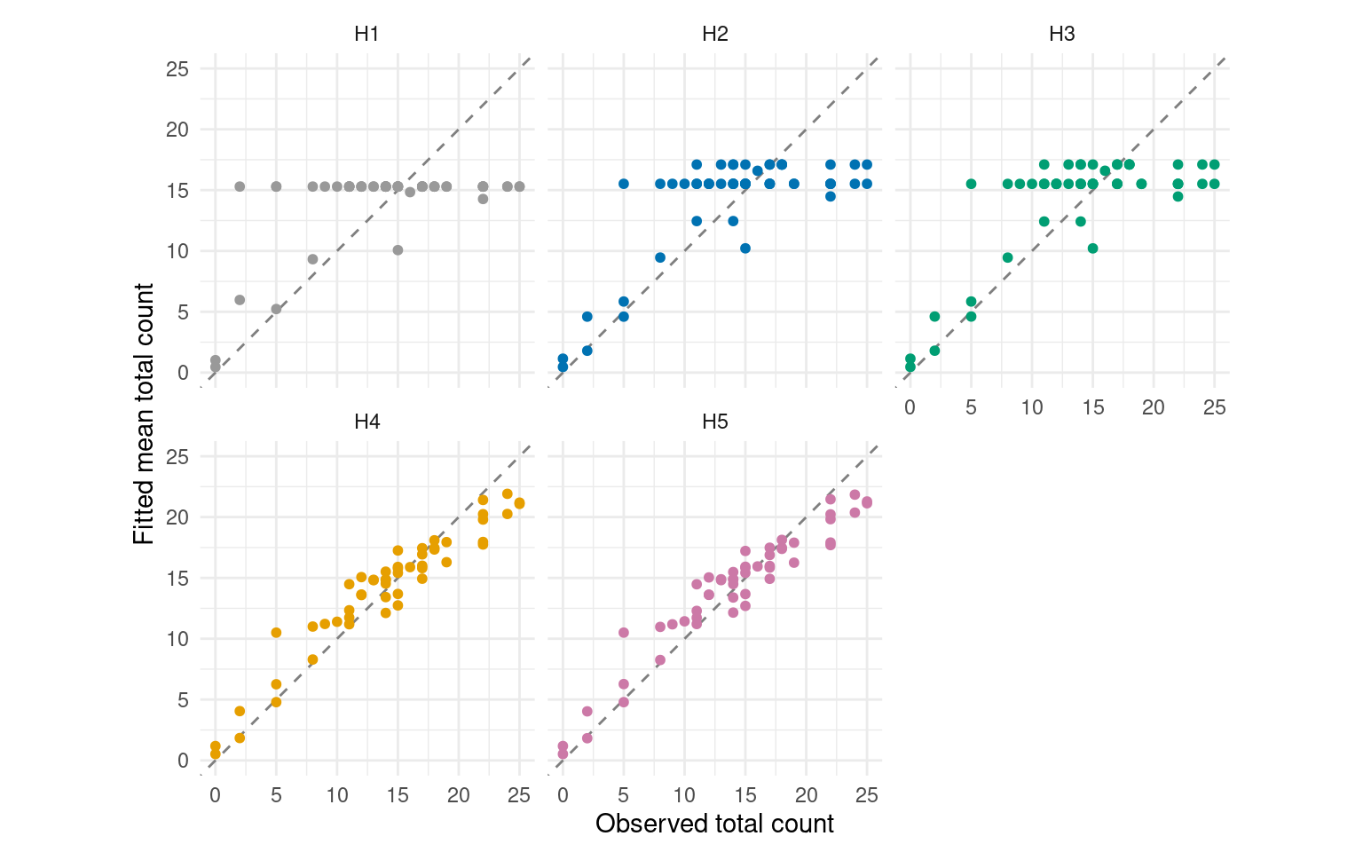
The horizontal bands in H1–H3 arise because equal-area portions have the same fitted count under H1, or the same count within a stratum under H2–H3. Smaller portions have correspondingly lower fitted counts. H4–H5 also allow magnitude to vary spatially, so their fitted counts follow the observed variation more closely. We next assess prediction at plots excluded from fitting.
Predict held-out plots
We assess prediction using leave-one-plot-out cross-validation of this first inventory. Each model is fitted to 47 plots and predicts the omitted plot, repeating this for all 48 plots. If a plot crosses a stratum boundary, all its portions are withheld together. The observed counts at that plot are used only to assess its predictions.
magCompCV() handles the refitting and prediction. We assign portions to folds using their original plot_id, and use the same model formulas and MCMC settings as above. The following call illustrates H5; cross_validate_ladder.R runs the comparison for any of H1–H5.
source("ladder_functions.R")
formulas <- ladder_formulas("H5")

portions <- trees |> distinct(unit_id, plot_id, area_ha)
fold_id <- setNames(portions$plot_id, portions$unit_id)

set.seed(1)
cv <- magCompCV(
  dat, magnitude = formulas$magnitude, composition = formulas$composition,
  fold_id = fold_id, target = "observation", type = "count", summary = "samples",
  control = magCompControl(
    n_samples = 50000, n_burn = 20000, n_thin = 10,
    n_chains = 3, n_cores = 3, chain_seeds = 1:3,
    nb_size = 1000, verbose = FALSE
  )
)
For each held-out plot, we sum its portions’ predicted counts within each draw and divide by their combined sampled area. Cross-validation uses all 3,000 retained draws per chain. summarize_ladder_cv.R compares these predictions with the observed species-by-DBH densities. Mean error indicates overprediction or underprediction, root mean squared prediction error (RMSPE) summarizes error magnitude, and coverage and width describe the pointwise 95% predictive intervals. Each of the 48 × 30 plot cells receives equal weight, including zero counts.
cv_summary <- read_csv("data/cv/summary.csv")

cv_summary |>
  select(model, mean_error, rmspe, coverage, mean_width) |>
  knitr::kable(digits = c(0, 2, 2, 1, 1), col.names = c(
    "Model", "Mean error (trees/ha)", "RMSPE (trees/ha)",
    "Coverage (%)", "Mean width (trees/ha)"
))| Model | Mean error (trees/ha) | RMSPE (trees/ha) | Coverage (%) | Mean width (trees/ha) |
|---|---|---|---|---|
| H1 | -0.04 | 42.61 | 96.7 | 77.6 |
| H2 | 0.04 | 41.80 | 96.7 | 76.4 |
| H3 | 0.02 | 41.30 | 96.7 | 78.1 |
| H4 | 0.09 | 40.82 | 97.0 | 80.8 |
| H5 | 0.12 | 40.07 | 97.5 | 90.5 |
H5 has the lowest RMSPE, about 6% below H1, but also the widest intervals. All five models have small mean errors and observed-cell coverage of about 97%. The added stratum and spatial structure therefore gives a modest improvement in prediction of the observed cell densities.
We also assess prediction within each stratum, scoring each held-out portion using its own counts and area. Each entry below gives RMSPE (trees/ha), with 95% predictive-interval coverage (%) in parentheses.
cv_strata <- read_csv("data/cv/stratum_summary.csv")

cv_strata |>
  mutate(score = sprintf("%.1f (%.1f)", rmspe, coverage)) |>
  select(stratum_id, portions, model, score) |>
  pivot_wider(names_from = model, values_from = score) |>
knitr::kable(col.names = c("Stratum", "Portions", paste0("H", 1:5)))| Stratum | Portions | H1 | H2 | H3 | H4 | H5 |
|---|---|---|---|---|---|---|
| 1 | 2 | 39.0 (95.0) | 36.7 (95.0) | 37.2 (95.0) | 36.9 (96.7) | 38.9 (93.3) |
| 2 | 16 | 48.4 (96.9) | 48.0 (97.3) | 46.8 (97.1) | 46.4 (97.1) | 45.1 (97.7) |
| 3 | 3 | 33.1 (100.0) | 20.5 (95.6) | 21.0 (95.6) | 21.1 (96.7) | 21.2 (96.7) |
| 4 | 31 | 40.5 (96.8) | 40.4 (96.7) | 40.1 (96.8) | 39.6 (97.2) | 39.2 (97.8) |
H5 has the lowest RMSPE in strata 2 and 4, while H2 has the lowest in strata 1 and 3. In the wetland stratum, adding stratum effects accounts for most of the improvement. Strata 1 and 3 have only two and three sampled portions, respectively, so these CV scores provide limited evidence for choosing among models. They assess prediction at withheld portions. The census comparisons below assess full-stratum estimates for this inventory, and the repeated-sampling study evaluates their estimation error and interval coverage across 1,000 layouts.
Predict the unsampled forest
Our target is stem density in this particular forest, expressed in trees per hectare. Because the sampled counts are known, each posterior draw of the forest total combines those observed counts with predicted counts in the unsampled area.
The square spatial prediction cells have nominal area m², equal to a full sampling plot. They are clipped to the forest, split at stratum boundaries, and have sampled areas removed. This leaves 1,515 unsampled portions. Their areas and the sampled areas sum to the full stratum areas.
We read these portions and generate joint predictions over the entire remainder. target = "observation" draws total counts and their species-by-DBH allocations, including uncertainty in model parameters and random effects. The spatial predictions also preserve dependence among prediction locations.
Add the observed counts
For each species-by-DBH cell, we add its observed count to every draw of its predicted unsampled count. standSummary(type = "total") multiplies predicted densities by their represented areas and sums within strata. We then add the observed counts using matching stratum and category labels.
unsampled <- standSummary(
  h5_predictions, data = prediction, unit = unit_id, group = stratum_id,
  represented_area = area_ha, type = "total", summary = "samples"
)

observed <- trees |>
  mutate(stratum = factor(stratum_id, levels = 1:4),
         category = paste(species, dbh_class, sep = ":"))
observed_counts <- xtabs(count ~ stratum + category, data = observed)

stratum_ids <- dimnames(unsampled$total)[[1]]
categories <- dimnames(unsampled$total)[[2]]
known_counts <- observed_counts[stratum_ids, categories]

# Dimensions are stratum x category x draw x chain.
h5_totals <- sweep(unsampled$total, c(1, 2), known_counts, "+")
For example, one draw for hemlock in the smallest DBH class in stratum 2 has the following contributions.
Summarize after aggregation
We divide population counts by the full stratum areas. Forest summaries sum stratum counts within each draw before division and interval calculation; adding interval endpoints would not give a forest interval.
areas <- setNames(stratum_areas$area_ha, stratum_areas$stratum_id)
stratum_density <- sweep(h5_totals, 1, areas[stratum_ids], "/")
forest_density <- apply(h5_totals, c(2, 3, 4), sum) / sum(areas)

forest_summary <- tibble(
  category = dimnames(forest_density)[[1]],
  mean = apply(forest_density, 1, mean),
  lower = apply(forest_density, 1, quantile, 0.025),
  upper = apply(forest_density, 1, quantile, 0.975)
)
The intervals summarize the posterior predictive distributions of census densities, conditional on the sampled trees and model assumptions.
Compare estimates with the census
We now use the full census to assess the estimates. Black horizontal marks show true densities; colored points and bars show posterior means and 95% intervals. Models are offset within each DBH class to keep their intervals visible.
comparison <- read_csv("data/ladder/comparison.csv")
cell_comparison <- comparison |>
  filter(target == "Species-by-DBH") |>
  separate_wider_delim(category, ":", names = c("species", "dbh_class")) |>
  mutate(species = factor(species, levels = species_order),
         dbh_class = ordered(dbh_class, levels = dbh_classes))
Forest stand table
Show plotting code
forest_comparison <- cell_comparison |> filter(domain == "Forest")

ggplot(forest_comparison, aes(dbh_class, mean, color = model)) +
  geom_errorbar(aes(ymin = lower, ymax = upper), width = 0,
                position = position_dodge(width = 0.7), alpha = 0.65) +
  geom_point(position = position_dodge(width = 0.7), size = 1.4) +
  geom_point(data = forest_comparison |> distinct(species, dbh_class, truth),
             aes(dbh_class, truth), inherit.aes = FALSE, shape = 95, size = 6) +
  facet_wrap(~ species, scales = "free_y", ncol = 3) +
  scale_color_manual(values = model_colors) +
  scale_y_continuous(limits = c(0, NA), expand = expansion(mult = c(.01, .08))) +
  labs(x = "DBH class (cm)", y = "Density (trees/ha)", color = "Model") +
  theme_minimal() +
  theme(legend.position = "bottom", axis.text.x = element_text(angle = 45, hjust = 1))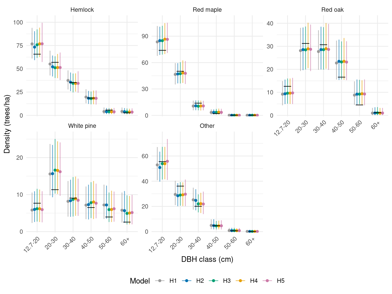
The forest estimates are similar across models in this sample. Each model’s interval for overall forest density includes the census value of 578.8 trees/ha.
Stratum stand tables
Stratum comparisons show differences that are less apparent after averaging over the whole forest.
Show plotting code
stand_comparison <- cell_comparison |> filter(domain != "Forest")

ggplot(stand_comparison, aes(dbh_class, mean, color = model)) +
  geom_errorbar(aes(ymin = lower, ymax = upper), width = 0,
                position = position_dodge(width = 0.7), alpha = 0.6) +
  geom_point(position = position_dodge(width = 0.7), size = 0.9) +
  geom_point(data = stand_comparison |> distinct(domain, species, dbh_class, truth),
             aes(dbh_class, truth), inherit.aes = FALSE, shape = 95, size = 4) +
  facet_wrap(~ domain + species, scales = "free_y", ncol = 5) +
  scale_color_manual(values = model_colors) +
  scale_y_continuous(limits = c(0, NA), expand = expansion(mult = c(.01, .08))) +
  labs(x = "DBH class (cm)", y = "Density (trees/ha)", color = "Model") +
  theme_minimal(base_size = 10) +
  theme(legend.position = "bottom", axis.text.x = element_text(angle = 60, hjust = 1))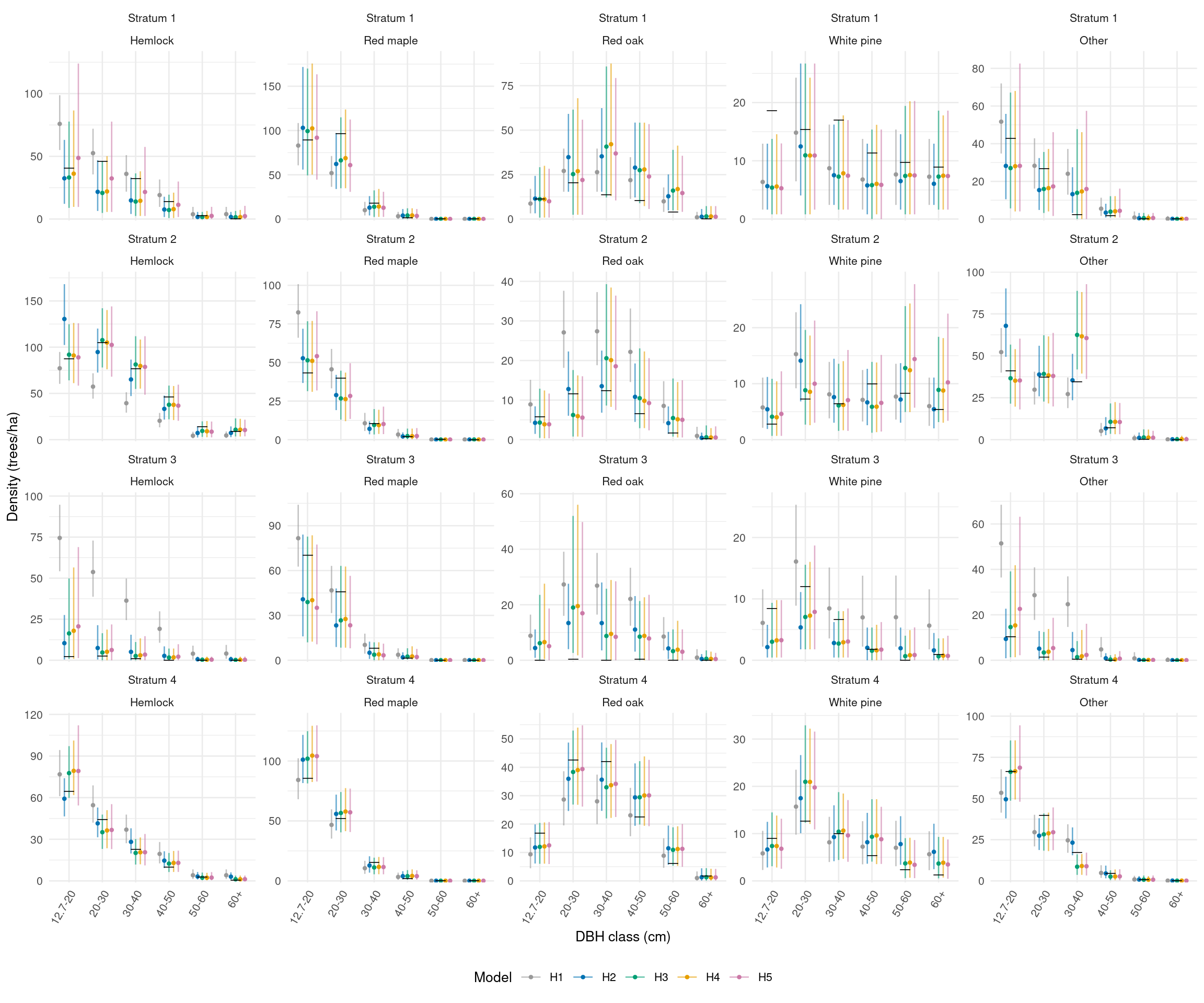
The wetland stratum has only nine sampled stems, all red maple or white pine, although other species occur in its census. A stratum factor can share information across strata, but cannot determine the missing species and size composition precisely. Wider intervals can be appropriate when this uncertainty is represented.
The common-intercept model cannot represent the wetland’s much lower expected stem density. H1 estimates about 590 trees/ha there, compared with census density of 174 trees/ha; H2 estimates about 181 trees/ha after adding stratum effects.
We also compare overall density, summing all species and DBH classes within each draw. This is a different, less detailed target than any individual stand-table cell.
Show plotting code
overall <- comparison |> filter(target == "Overall density")

ggplot(overall, aes(model, mean, color = model)) +
  geom_hline(data = overall |> distinct(domain, truth),
              aes(yintercept = truth), linetype = "dashed") +
  geom_errorbar(aes(ymin = lower, ymax = upper), width = 0.15) +
  geom_point(size = 1.8) +
  facet_wrap(~ domain, scales = "free_y", ncol = 3) +
  scale_color_manual(values = model_colors, guide = "none") +
  labs(x = "Model", y = "Overall density (trees/ha)") +
  theme_minimal()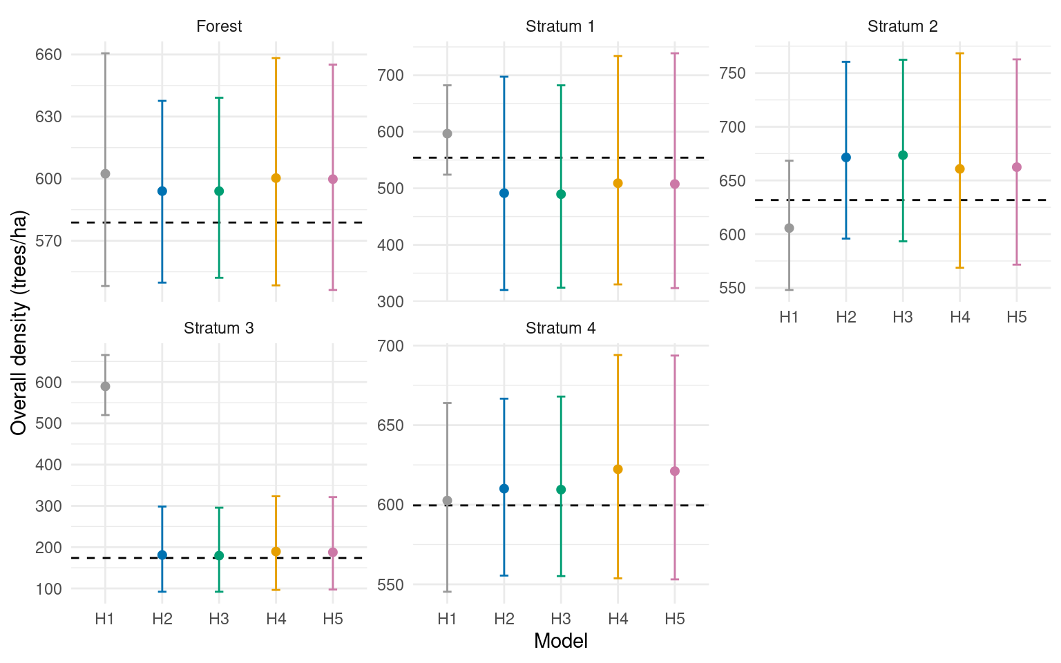
We next repeat the sampling to assess how these estimates and intervals behave as the inventory changes.
Repeated sampling of the same forest
We hold the census, boundaries, DBH classes, and nominal prediction-cell areas fixed and change the random shift of the sampling grid. Each layout gives a new inventory to which all five models are fitted. Sampled areas are removed from the prediction cells separately for each inventory.
Each fit provides Bayesian inference conditional on its sample and model. The experiment evaluates these estimates and intervals as the sample changes, following the distinction between Bayesian inference and repeated-sampling assessment discussed by Little (2012). A 95% posterior interval need not have 95% repeated-sampling coverage for every fixed forest, especially when the model misses features of that population. We do not simulate new forests from the fitted model.
The results below summarize 1,000 random sampling layouts, including the first inventory illustrated above. All five models use the same sample within each layout and the MCMC settings given above. The download’s README provides instructions for reproducing the experiment and details of the chain diagnostics.
Stand-table accuracy and interval coverage
Here, repeated-sampling bias is estimated by averaging each inventory’s posterior mean estimate minus the fixed census value across plot layouts. Positive values indicate overestimation on average; negative values indicate underestimation. Design-unbiasedness would require the average error over all possible layouts under the sampling design to be zero. Our posterior means are not constructed to guarantee that property; we are measuring their performance for this forest and sampling design.
Relative bias expresses the average error as a percentage of the true density. RMSE describes error magnitude, coverage is the percentage of intervals containing the fixed census value, and width summarizes interval length.
The figure summarizes the 30 species-by-DBH cells within each reporting area, including cells with zero census counts. RMSE uses their squared errors; coverage and width average across cells. Bars show Monte Carlo standard errors calculated across inventories.
Show plotting code
repeated_summary <- read_csv("data/repeated_ladder/domain_summary.csv")

metric_plot <- repeated_summary |>
  filter(target == "Species-by-DBH") |>
  select(domain, model, rmse, coverage, mean_width, rmse_mcse, coverage_mcse, width_mcse) |>
  pivot_longer(c(rmse, coverage, mean_width), names_to = "metric", values_to = "value") |>
  mutate(mcse = case_when(metric == "rmse" ~ rmse_mcse,
                          metric == "coverage" ~ coverage_mcse,
                          metric == "mean_width" ~ width_mcse),
         metric = factor(metric, levels = c("rmse", "coverage", "mean_width"),
           labels = c("RMSE (trees/ha)", "Coverage (%)", "Width (trees/ha)")))

ggplot(metric_plot, aes(model, value, color = model)) +
  geom_hline(data = metric_plot |> filter(metric == "Coverage (%)") |>
               distinct(domain, metric) |> mutate(reference = 95),
             aes(yintercept = reference),
             linetype = "dashed", color = "grey50") +
  geom_errorbar(aes(ymin = value - mcse, ymax = value + mcse), width = 0.15) +
  geom_point(size = 1.5) +
  facet_wrap(~ domain + metric, scales = "free_y", ncol = 3) +
  scale_color_manual(values = model_colors, guide = "none") +
  labs(x = "Model", y = NULL) +
  theme_minimal(base_size = 10)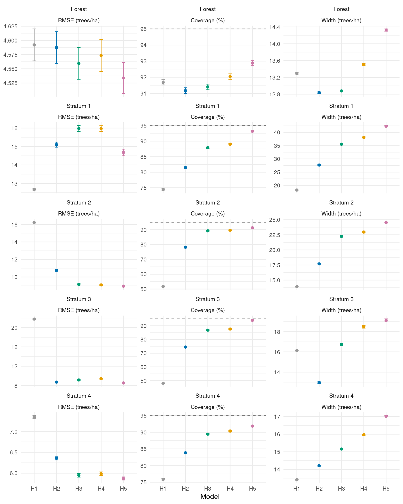
Forest-level RMSE is similar across the five models. The benefits of allowing more local variation are clearer within strata. Adding stratum effects to magnitude and species allocation (H1 to H2) substantially reduces RMSE in strata 2–4 and improves coverage in all four strata.
Allowing DBH allocation within species to vary by stratum (H2 to H3) further improves coverage, although RMSE improves in some strata and increases in others. Adding a spatial magnitude effect (H3 to H4) makes little further difference. Adding the species spatial factor (H4 to H5) reduces RMSE and improves coverage in every stratum. H5’s average cell coverage ranges from about 91% to 94%, compared with 48% to 76% for H1. The richer models therefore provide a clearer improvement in stratum-level uncertainty reporting than in forest-level point estimates.
Stratum 1 illustrates why additional complexity is not always better for point estimation. H1 has lower RMSE than H5 there (12.7 versus 14.7 trees/ha), but its coverage is only about 74%, compared with 93% for H5. H5’s wider intervals better reflect estimation error across these layouts. Low coverage means that intervals exclude the census values too often, so RMSE alone would miss this difference. These rates average across the 30 stand-table cells; individual species and DBH classes can perform differently.
Overall density
Overall density is assessed after summing species and DBH counts within every predictive draw. For the forest as a whole, all five models have relative biases below 1% in magnitude. Values in parentheses below are Monte Carlo standard errors across the 1,000 layouts.
repeated_summary |>
  filter(target == "Overall density", domain == "Forest") |>
  transmute(
    Model = model,
    `Relative bias (%)` = sprintf("%.2f (%.2f)", relative_bias, relative_bias_mcse),
    `RMSE (trees/ha)` = sprintf("%.1f (%.1f)", rmse, rmse_mcse),
    `Coverage (%)` = sprintf("%.1f (%.1f)", coverage, coverage_mcse),
    `Width (trees/ha)` = sprintf("%.1f (%.1f)", mean_width, width_mcse)
  ) |>
knitr::kable()| Model | Relative bias (%) | RMSE (trees/ha) | Coverage (%) | Width (trees/ha) |
|---|---|---|---|---|
| H1 | 0.03 (0.11) | 19.5 (0.4) | 99.6 (0.2) | 129.0 (0.4) |
| H2 | -0.07 (0.11) | 20.1 (0.5) | 96.8 (0.6) | 87.5 (0.1) |
| H3 | -0.07 (0.11) | 20.1 (0.5) | 96.9 (0.5) | 87.6 (0.1) |
| H4 | 0.78 (0.10) | 19.5 (0.4) | 100.0 (0.0) | 130.5 (0.5) |
| H5 | 0.78 (0.10) | 19.4 (0.4) | 100.0 (0.0) | 130.8 (0.5) |
Forest overall-density intervals are conservative under this sampling design, with coverage from 96.8% to 100%. H2 and H3 give narrower intervals than the other models with similar RMSE. This differs from the cell-level comparison above: summing categories changes both the target and its uncertainty.
Stratum totals can behave differently. H1 substantially overestimates wetland density because it applies a common magnitude across the forest. Stratum effects greatly reduce that error, but wetland relative bias remains about 16% for H2 and H3 and 24% for H4 and H5. H5’s 95.1% coverage for overall wetland density accompanies wide intervals; it does not mean the point estimates are unbiased. Sparse observations and a model’s ability to describe the population both matter.
What this example establishes
Across repeated samples, similar forest-level RMSE conceals important differences within strata. Stratum effects account for much of the improvement in local point estimates, while the DBH stratum factor and species spatial factor improve interval coverage. H1 still gives lower RMSE in stratum 1. Additional complexity therefore needs to be assessed for the intended reporting areas, considering estimation error, interval coverage, and interval width together.
Cross-validation checks prediction at omitted plots. The census comparisons assess forest and stratum estimates formed by combining observed counts with predictions for unsampled areas. Repeating the inventory shows how those estimates behave as the sample changes. These assessments complement one another: similar plot-level scores or forest averages can conceal differences that matter for local stand tables.