A stand table describes how trees are distributed among species and diameter classes, usually in trees per hectare. We estimate a forest stand table by combining a magnitude model for overall tree density, a composition model for species, and a conditional composition model for diameter at breast height (DBH) within each species. Using the shared simulated forest, we fit all three components, examine parameter estimates and fitted values, and compare predicted forest species-by-DBH densities with truth.
The magnitude article and composition article explain the individual components. The DBH article combines magnitude and DBH allocation after summing over species. Here we retain species information and add a second allocation within each species to describe its DBH distribution. The magnitude model predicts total counts at new locations, and the composition models allocate them among species and then DBH classes. We therefore do not need to supply known prediction-cell totals.
Example data
Download the plot-sampling data (ZIP)
The introductory plot-sampling articles use this same archive. Extract it and use the folder containing data/ as your R working directory.
Read the data
The shared data contain 151 sampled plots and 4,812 prediction cells, with simulated counts for pine, oak, and birch in five DBH classes. Each class includes its lower bound and excludes its upper bound; 50+ includes trees at least 50 cm in diameter. The predictor x is p95 canopy height standardized using the plots’ mean and standard deviation.
We read the plot and prediction tables, then arrange the plot counts into one row per plot, species, and DBH class. Zero counts remain in the table.
library(magComp)
library(tidyverse)

set.seed(1)

plots <- read_csv("data/plots.csv")

prediction <- read_csv("data/prediction.csv")

species_order <- c("pine", "oak", "birch")
dbh_classes <- c("10-20", "20-30", "30-40", "40-50", "50+")

trees <- plots |>
  select(plot_id, area, x, contains(":")) |>
  pivot_longer(contains(":"), names_to = c("species", "dbh_class"),
               names_sep = ":", values_to = "count") |>
  mutate(
    species = factor(species, levels = species_order),
    dbh_class = ordered(dbh_class, levels = dbh_classes)
  ) |>
  arrange(plot_id, species, dbh_class)

trees |>
  filter(plot_id == 1) |>
  knitr::kable(digits = 3)
| 1 |
0.126 |
-0.811 |
pine |
10-20 |
6 |
| 1 |
0.126 |
-0.811 |
pine |
20-30 |
3 |
| 1 |
0.126 |
-0.811 |
pine |
30-40 |
6 |
| 1 |
0.126 |
-0.811 |
pine |
40-50 |
3 |
| 1 |
0.126 |
-0.811 |
pine |
50+ |
2 |
| 1 |
0.126 |
-0.811 |
oak |
10-20 |
4 |
| 1 |
0.126 |
-0.811 |
oak |
20-30 |
8 |
| 1 |
0.126 |
-0.811 |
oak |
30-40 |
2 |
| 1 |
0.126 |
-0.811 |
oak |
40-50 |
1 |
| 1 |
0.126 |
-0.811 |
oak |
50+ |
0 |
| 1 |
0.126 |
-0.811 |
birch |
10-20 |
15 |
| 1 |
0.126 |
-0.811 |
birch |
20-30 |
4 |
| 1 |
0.126 |
-0.811 |
birch |
30-40 |
1 |
| 1 |
0.126 |
-0.811 |
birch |
40-50 |
0 |
| 1 |
0.126 |
-0.811 |
birch |
50+ |
0 |
Each plot has 15 species-by-DBH counts. Their sum gives its total tree count; summing within species gives the species totals.
How the model components fit together
For plot , let be its total tree count, its sampled area in hectares, and its expected density in trees/ha. The magnitude model is
where the negative-binomial distribution has mean and size . The generating values are , , and . Thus, expected density at average plot p95 is 350 trees/ha.
Let denote species and denote DBH class. Write for the probability of species and for the probability of DBH class within that species. The species probabilities denoted in the composition article are now ; we use for the joint species-by-DBH probability,
Species probabilities sum to one, and DBH probabilities sum to one within each species. The 15 joint probabilities therefore sum to one. Conditional on , the counts follow a multinomial distribution with those probabilities. For species and DBH class , expected density is and expected plot count is .
Both composition components use sequential probit allocation. Trees are allocated to pine, then oak, with birch receiving the remainder. Within each species, allocation proceeds through the DBH classes from smallest to largest. Each allocation step has its own intercept and canopy-height slope, with pnorm() converting their linear expression to a conditional probability. The last DBH class receives the remaining trees of that species.
The species and DBH models have separate regression coefficients, denoted by . Each species has its own set of DBH coefficients. We use the same predictor x in all components; the formulas also allow different predictors for magnitude, species, and conditional DBH composition.
Fit the full model
We supply the category columns in species-then-DBH order. species ~ x specifies species allocation, and dbh_class | species ~ x specifies DBH allocation within each species.
dat <- magCompData(
  trees,
  unit = plot_id, categories = c(species, dbh_class),
  tree_count = count, design = fixedArea(area)
)

fit <- magComp(
  dat,
  magnitude = ~ x,
  composition = magCompComposition(
    species ~ x,
    dbh_class | species ~ x
  ),
  control = magCompControl(
    n_samples = 2000,
    n_burn = 1000,
    n_chains = 3,
    n_cores = 3,
    chain_seeds = 1:3,
    verbose = FALSE
  )
)
The factor levels specify the allocation sequences. Ordering the DBH factor does not by itself smooth coefficients across classes; this example uses independent Normal coefficient priors. Negative-binomial size is estimated under its default Gamma prior with shape 1 and rate 0.01. We retain the automatic starting values.
Each of three MCMC chains runs for 2,000 iterations and discards the first 1,000. We use all 3,000 retained draws for parameter summaries.
Magnitude and species parameters
We use summary() to obtain posterior estimates, 95% credible intervals, and chain diagnostics, then add the generating values from the data article.
parameter_summary <- summary(fit)

# Magnitude rows are the intercept, canopy-height slope, and size.
magnitude_summary <- parameter_summary |>
  filter(component == "magnitude") |>
  mutate(truth = c(log(350), -0.2, 50))

true_alpha <- c("pine:(Intercept)" = 0, "pine:x" = 0.5,
                "oak:(Intercept)" = -0.5, "oak:x" = -0.5)

species_summary <- parameter_summary |>
  filter(block == "species") |>
  mutate(truth = true_alpha[index])

bind_rows(magnitude_summary, species_summary) |>
  select(symbol, truth, mean, q2_5, q97_5, rhat, ess) |>
  knitr::kable(
    digits = 3,
    col.names = c("Parameter", "Truth", "Mean", "2.5%", "97.5%", "R-hat", "ESS")
  )
| beta[0] |
5.858 |
5.856 |
5.823 |
5.889 |
1.000 |
2764.501 |
| beta[x] |
-0.200 |
-0.186 |
-0.218 |
-0.155 |
1.001 |
2762.898 |
| r_M |
50.000 |
66.148 |
37.105 |
124.010 |
1.000 |
313.055 |
| alpha[0,pine] |
0.000 |
0.009 |
-0.022 |
0.041 |
1.000 |
1177.263 |
| alpha[x,pine] |
0.500 |
0.492 |
0.458 |
0.527 |
1.000 |
905.293 |
| alpha[0,oak] |
-0.500 |
-0.508 |
-0.560 |
-0.454 |
1.002 |
615.524 |
| alpha[x,oak] |
-0.500 |
-0.500 |
-0.550 |
-0.451 |
1.000 |
611.056 |
beta[0] is log expected density at average plot p95, and beta[x] is its change for a one-standard-deviation increase in p95. Exponentiating the slope gives the corresponding multiplier on density. The species alpha coefficients describe conditional probit probabilities, as in the composition article. R-hat values near one indicate agreement among chains; ESS is the effective sample size after accounting for dependence among draws.
DBH allocation coefficients
There are 24 DBH coefficients, an intercept and slope for each of four allocation steps within each of three species. We arrange their generating values as a table and match them to the fitted parameter labels.
true_dbh <- tibble(
  species = rep(species_order, each = 4),
  dbh_class = rep(dbh_classes[1:4], times = 3),
  intercept = c(-1, -0.5, 0, 0.5,
                -0.5, 0, 0.5, 1,
                 0, 0.5, 1, 1.5),
  slope = c(-0.4, -0.3, -0.2, -0.1,
            -0.3, -0.3, -0.2, -0.2,
            -0.2, -0.2, -0.1, -0.1)
) |>
  pivot_longer(c(intercept, slope), names_to = "coefficient",
               values_to = "truth") |>
  mutate(index = paste(species, dbh_class,
                        if_else(coefficient == "intercept", "(Intercept)", "x"),
                        sep = ":"))

dbh_summary <- parameter_summary |>
  filter(block == "dbh_class|species") |>
  left_join(true_dbh, by = "index") |>
  mutate(
    species = factor(species, levels = species_order),
    dbh_class = ordered(dbh_class, levels = dbh_classes[1:4]),
    coefficient = factor(coefficient, levels = c("intercept", "slope"),
                          labels = c("Intercept", "Canopy-height slope"))
  )
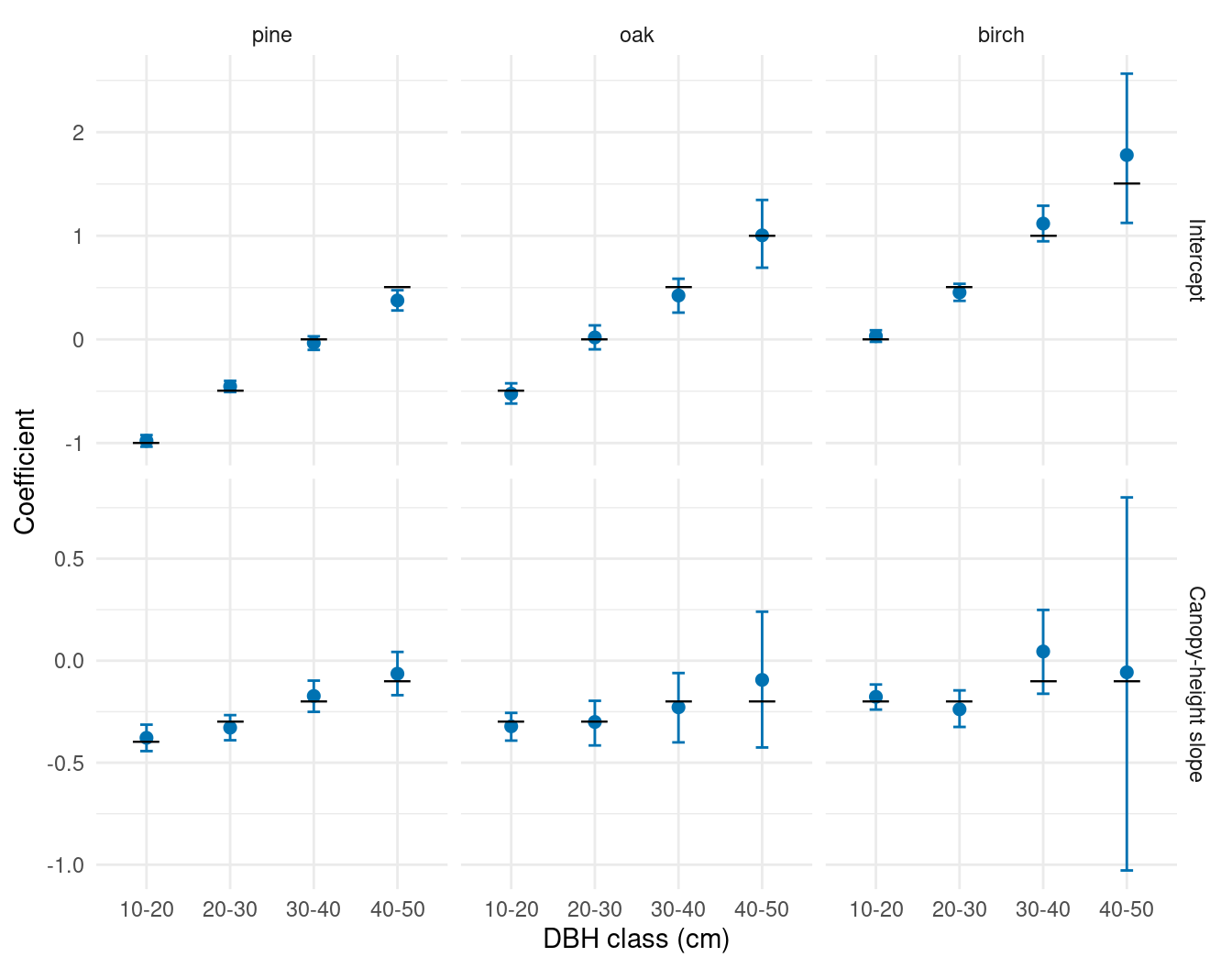
We compare the estimated coefficients and intervals with truth. A DBH slope describes allocation to that class among the trees of the species still available after earlier classes.
ggplot(dbh_summary, aes(dbh_class, mean)) +
  geom_errorbar(aes(ymin = q2_5, ymax = q97_5), width = 0.15,
                color = "#0072B2") +
  geom_point(color = "#0072B2", size = 2) +
  geom_point(aes(y = truth), shape = 95, size = 6) +
  facet_grid(coefficient ~ species, scales = "free_y") +
  labs(x = "DBH class (cm)", y = "Coefficient") +
  theme_minimal()
The later birch allocation steps have wider intervals because relatively few birch trees remain to inform those coefficients.
Across the 31 parameters, the largest R-hat is 1.01 and the smallest ESS is about 266. Trace plots are available with plot(fit) when examining individual chains.
Examine fitted values
For a full model, fitted(fit) returns posterior means for overall density, joint category probabilities, category densities, and category counts. Here we request category densities and arrange the first plot’s fitted values as a stand table.
fitted_mean <- fitted(fit, type = "density")

# Category columns follow DBH class within species.
first_plot <- matrix(
  fitted_mean$density[1, ], nrow = length(dbh_classes),
  dimnames = list(dbh_classes, species_order)
)

knitr::kable(first_plot, digits = 1)
| 10-20 |
35.5 |
48.2 |
81.6 |
| 20-30 |
45.1 |
44.3 |
45.7 |
| 30-40 |
33.0 |
21.2 |
13.7 |
| 40-50 |
18.6 |
6.8 |
2.1 |
| 50+ |
9.3 |
1.1 |
0.1 |
Entries are fitted densities in trees/ha. Their sum is the fitted overall density for that plot. These are expected densities under the fitted model; the observed counts divided by plot area fluctuate around them.
Predict and aggregate across the forest
For each selected posterior draw, prediction first generates a total count from the negative-binomial model at each cell. It then allocates the count among species and DBH classes. type = "density" returns those counts divided by cell area. We supply only IDs, canopy height, and cell areas; the simulated cell counts are reserved for comparison with truth.
predictions <- predict(
  fit,
  prediction |> select(plot_id, x, area),
  type = "density",
  target = "observation",
  n_draws = 100,
  summary = "samples"
)

# Prediction cell x species-by-DBH category x retained draw x chain.
dim(predictions$density)
#> [1] 4812   15  100    3
The array contains 4,812 cells, 15 categories, 100 retained draws, and three chains. These draws include parameter uncertainty and variation in both total counts and their allocation.
We use standSummary() to average densities across the forest within each draw, weighting by cell area. Smaller boundary cells contribute less to the forest average. Omitting group produces a forest-wide summary.
forest_predictions <- standSummary(
  predictions,
  data = prediction,
  unit = plot_id,
  represented_area = area,
  summary = "samples"
)

forest_summary <- summary(forest_predictions)

forest_estimates <- forest_summary |>
  as_tibble() |>
  separate_wider_delim(category, delim = ":", names = c("species", "dbh_class")) |>
  mutate(
    species = factor(species, levels = species_order),
    dbh_class = ordered(dbh_class, levels = dbh_classes)
  )

forest_estimates |>
  select(dbh_class, species, mean) |>
  pivot_wider(names_from = species, values_from = mean) |>
  arrange(dbh_class) |>
  knitr::kable(digits = 1)
| 10-20 |
25.8 |
59.9 |
56.6 |
| 20-30 |
40.3 |
31.8 |
33.7 |
| 30-40 |
43.2 |
12.8 |
13.7 |
| 40-50 |
32.5 |
4.3 |
2.0 |
| 50+ |
18.9 |
0.8 |
0.1 |
This is the estimated forest stand table in trees/ha. Each entry is a posterior predictive mean. We calculate intervals from the aggregated draws, including both count variation and parameter uncertainty.
Compare species-by-DBH distributions with truth
The true forest density for each species-by-DBH category is its simulated count summed over prediction cells, divided by their combined area. This is the same area-weighted density calculation used for predictions.
forest_truth <- prediction |>
  select(contains(":")) |>
  pivot_longer(everything(), names_to = c("species", "dbh_class"),
               names_sep = ":", values_to = "count") |>
  group_by(species, dbh_class) |>
  summarise(truth = sum(count) / sum(prediction$area), .groups = "drop")

comparison <- forest_estimates |>
  left_join(forest_truth, by = c("species", "dbh_class")) |>
  mutate(
    species = factor(species, levels = species_order),
    dbh_class = ordered(dbh_class, levels = dbh_classes)
  )
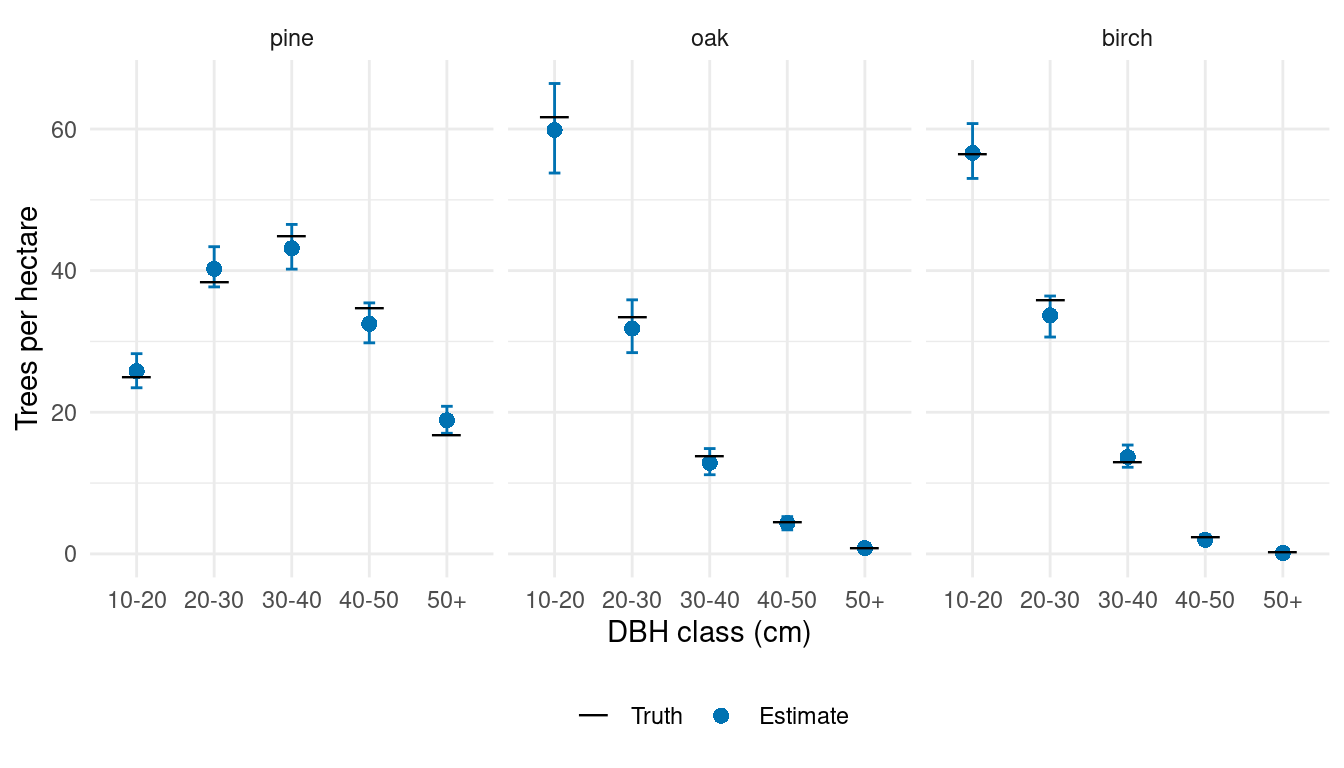
We plot each species’ DBH distribution using separate estimates for the diameter classes. Black horizontal marks show the realized forest densities from the simulated population.
ggplot(comparison, aes(dbh_class, mean)) +
  geom_errorbar(aes(ymin = q2_5, ymax = q97_5), width = 0.15,
                color = "#0072B2") +
  geom_point(aes(shape = "Estimate"), color = "#0072B2", size = 2.5) +
  geom_point(aes(y = truth, shape = "Truth"), size = 6) +
  scale_shape_manual(values = c("Truth" = 95, "Estimate" = 16),
                     breaks = c("Truth", "Estimate"), name = NULL) +
  facet_wrap(~ species, nrow = 1) +
  scale_y_continuous(limits = c(0, NA)) +
  labs(x = "DBH class (cm)", y = "Trees per hectare") +
  theme_minimal() +
  theme(legend.position = "bottom")
The estimates follow the main features of the simulated distributions. Pine is most abundant in the middle DBH classes, while oak and birch are concentrated in the smaller classes. The intervals describe uncertainty in the forest’s species-by-DBH densities, including uncertainty about total abundance. Within each draw, species and DBH allocations sum to that draw’s overall density.
The same predictions can produce stand tables by supplying the cell–stand area table to standSummary() with group = stand_id, as in the magnitude article. Summaries by species or DBH class are obtained by adding the relevant category densities within each draw before calculating intervals.
The next article adds stratum-specific intercepts to describe differences among groups of stands; its companion also allows canopy-height slopes to vary. Later articles introduce spatial effects, effects in within-species DBH allocation, and space-time effects. Each extension uses its own simulated population in the same forest.