We begin with a magnitude-only model to estimate overall tree density in trees per hectare. Using the shared simulated forest, we fit the model, examine fitted values, and aggregate predictions for the forest and its stands. Known population values let us assess parameter and density estimates. Comparisons with an intercept-only model and a direct estimate show what canopy height contributes. Subsequent articles consider composition alone and then combine magnitude and composition to estimate DBH distributions and species-by-DBH stand tables.
Example data
Download the plot-sampling data (ZIP)
The introductory plot-sampling articles use this same archive. Extract it and use the folder containing data/ as your R working directory.
Read the data
The shared data use real forest boundaries, plot locations, and UAV-derived canopy heights from Weisse Krug in Germany (Spitta et al. 2026). Tree counts are simulated. There are 151 sampled plots and 4,812 prediction cells; a full plot or cell covers approximately 0.126 ha, with smaller areas along the forest boundary.
We read the forest polygon and both data tables.
| 1 |
0.126 |
22.953 |
-0.811 |
55 |
| 2 |
0.123 |
24.860 |
-0.356 |
57 |
| 3 |
0.110 |
23.583 |
-0.661 |
37 |
| 4 |
0.126 |
26.102 |
-0.059 |
52 |
| 5 |
0.126 |
20.821 |
-1.320 |
48 |
| 6 |
0.120 |
23.326 |
-0.722 |
41 |
count is the total number of trees, area is the sampled area in hectares, and p95 is the 95th percentile of canopy-height model values in meters. The column x contains p95 standardized using the plots’ mean and standard deviation. Those same scaling values were applied to the prediction cells. We fit using the plot counts; simulated prediction-cell counts provide truth for assessment.
Define and fit the model
For plot , let be the observed count, its area in hectares, and the expected tree density in trees per hectare. We relate density to standardized canopy height and model counts with a negative-binomial (NB) distribution,
where is the mean count and is the size parameter. Larger plots have more expected trees at the same density. Count variance is , so a larger size parameter means less variation around the mean.
The intercept is log expected density at the plots’ average p95, and describes the change in log density for a one-standard-deviation increase in p95. In the technical document, the magnitude predictors here are . The data were generated with , , and . These values are known for comparison; the fit estimates all three parameters.
We supply the counts and areas with magCompData(). The formula ~ x includes an intercept and a canopy-height slope, while composition = NULL requests a magnitude-only model.
dat <- magCompData(plots, unit = plot_id, tree_count = count,
                   design = fixedArea(area))

fit <- magComp(
  dat,
  magnitude = ~ x,
  composition = NULL,
  control = magCompControl(
    n_samples = 2000,
    n_burn = 1000,
    n_chains = 3,
    n_cores = 3,
    chain_seeds = 1:3,
    verbose = FALSE
  )
)
Markov chain Monte Carlo (MCMC) produces parameter draws representing uncertainty given the data and priors. Each chain runs for 2,000 iterations, discards the first 1,000, and retains 1,000 draws, giving 3,000 draws across the three chains. We request three cores to run the chains in parallel and set their seeds for reproducibility. We use default priors and starting values. With no magnitude random effects, size is estimated automatically under a Gamma prior with shape 1 and rate 0.01; its hyperparameters can be changed with magCompPriors().
Parameter estimates
We use summary() to obtain parameter estimates and diagnostics, then add the generating values for comparison.
parameter_summary <- summary(fit)

# Rows are the intercept, standardized p95 slope, and size.
parameter_summary$truth <- c(log(350), -0.2, 50)

parameter_summary |>
  select(symbol, truth, mean, q2_5, q97_5, rhat, ess) |>
  knitr::kable(
    digits = 3,
    col.names = c("Parameter", "Truth", "Mean", "2.5%", "97.5%", "R-hat", "ESS")
  )
| beta[0] |
5.858 |
5.857 |
5.826 |
5.889 |
1 |
2430.399 |
| beta[x] |
-0.200 |
-0.186 |
-0.219 |
-0.153 |
1 |
2594.612 |
| r_M |
50.000 |
65.721 |
39.416 |
113.173 |
1 |
505.965 |
The labels beta[0], beta[x], and r_M correspond to , , and . The posterior mean summarizes each parameter’s draws; the 2.5% and 97.5% columns bound its central 95% credible interval. All three generating values fall within these intervals. Exponentiating a slope draw gives the corresponding multiplicative change in expected density for a one-standard-deviation increase in p95.
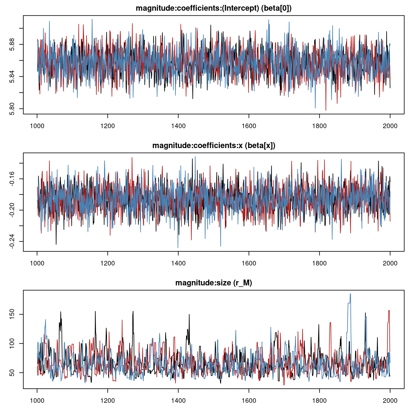
R-hat values near one indicate agreement among chains. ESS is the effective sample size, accounting for dependence among iterations. We also inspect the traces: the chains should overlap without a clear upward or downward trend.
plot(fit, n_col = 1, n_row = 3)
Examine fitted values
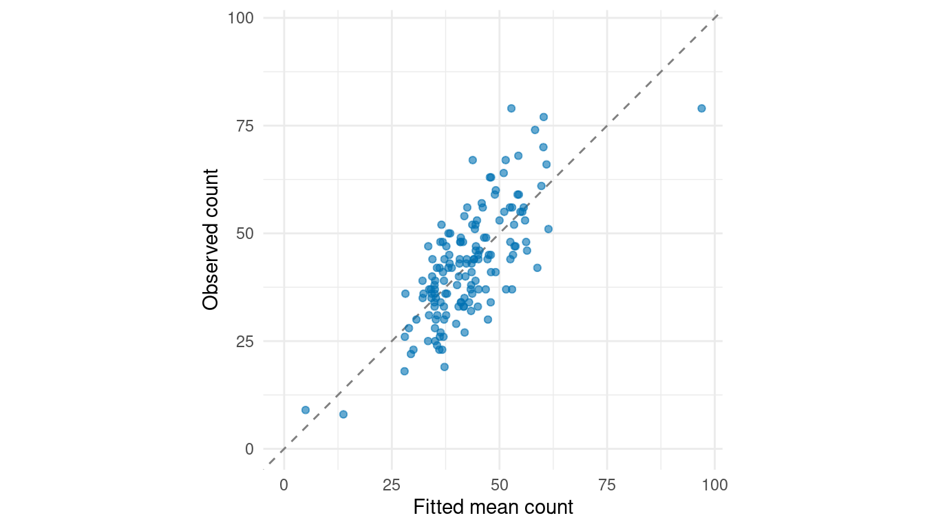
By default, fitted() returns posterior means of expected density as magnitude and expected count as count. We compare these values with the observed counts at the sampled plots.
fitted_mean <- fitted(fit)

fitted_values <- tibble(
  plot_id = plots$plot_id,
  observed_count = plots$count,
  expected_count = fitted_mean$count[, "total"],
  expected_density = fitted_mean$magnitude[, "total"]
)

fitted_values |>
  head() |>
  knitr::kable(digits = 1)
| 1 |
55 |
51.1 |
406.7 |
| 2 |
57 |
45.9 |
373.7 |
| 3 |
37 |
43.3 |
395.5 |
| 4 |
52 |
44.4 |
353.6 |
| 5 |
48 |
56.2 |
447.2 |
| 6 |
41 |
48.0 |
400.0 |
The table gives counts per plot and densities in trees/ha. We plot observed counts against fitted mean counts; the dashed line marks equality.
# Use the same count range on both axes, including zero.
count_limits <- range(0, fitted_values$expected_count, fitted_values$observed_count)

ggplot(fitted_values, aes(expected_count, observed_count)) +
  geom_abline(intercept = 0, slope = 1, linetype = "dashed", color = "grey50") +
  geom_point(color = "#0072B2", alpha = 0.6) +
  coord_equal(xlim = count_limits, ylim = count_limits) +
  labs(x = "Fitted mean count", y = "Observed count") +
  theme_minimal()
Counts vary around their means, so scatter is expected even when the model is correct. A systematic pattern above or below the line can indicate underprediction or overprediction. For additional diagnostics, ppcSummary(fit) compares observed counts with posterior predictive replicates and reports two-sided Bayesian posterior predictive p-values (Gelman, 2013). Small values flag unusual counts under the model; they are not probabilities that the model is correct.
Predict across the forest
To estimate realized forest density, we use posterior predictive counts. For each selected parameter draw, target = "observation" draws a count from the NB distribution at every prediction cell. This includes count variation as well as uncertainty in the coefficients and size. The function returns both these counts and their densities, obtained by dividing by cell area. We use 100 parameter draws per chain for prediction and retain the resulting predictive draws for aggregation. The fitted object still holds all draws for parameter summaries and diagnostics.
predictions <- predict(
  fit,
  prediction |> select(plot_id, x, area),
  target = "observation",
  n_draws = 100,
  summary = "samples"
)

# Prediction location x retained draw x chain.
dim(predictions$magnitude)
#> [1] 4812  100    3
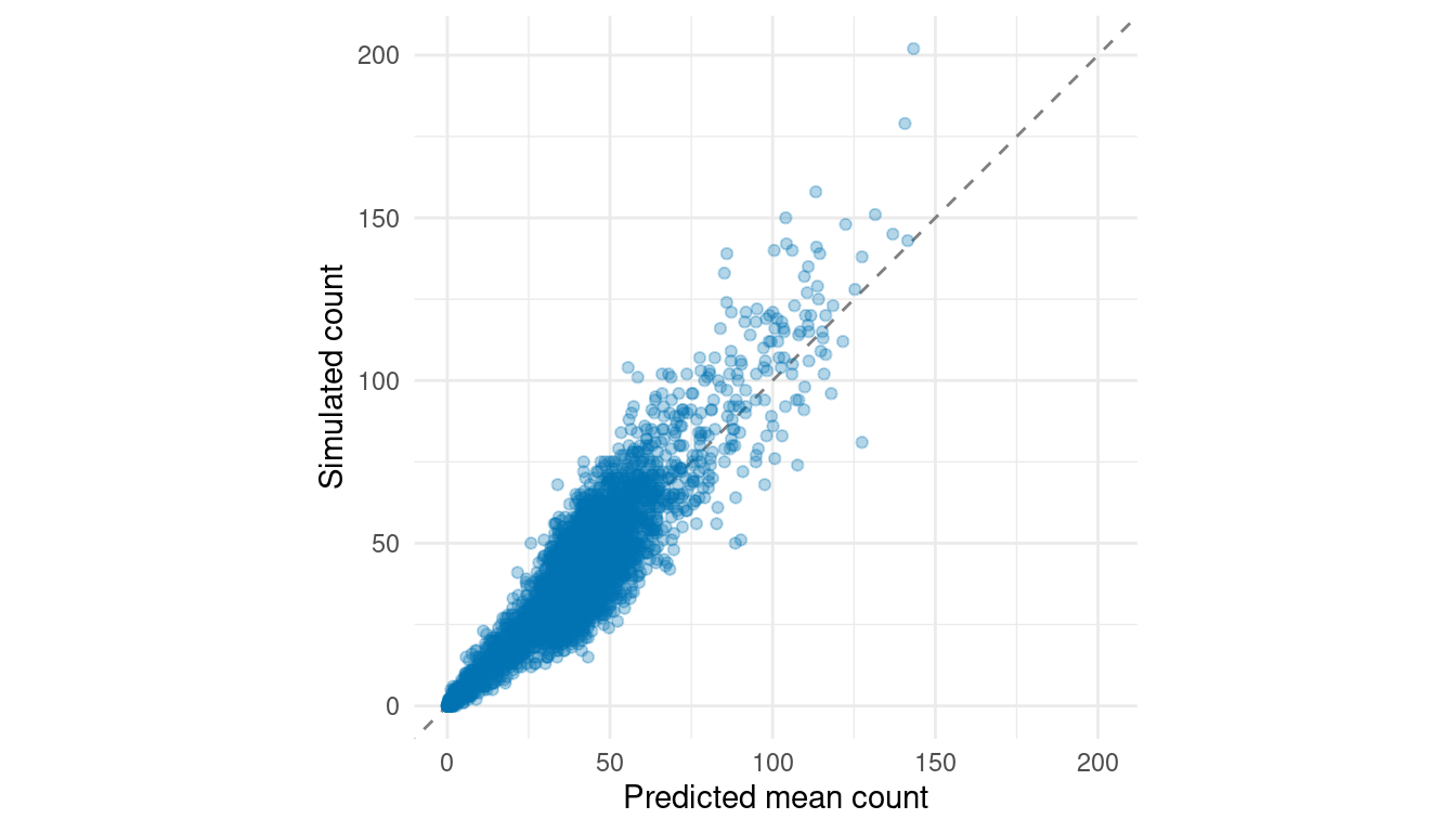
The magnitude array contains 4,812 locations, 100 draws per chain, and three chains. Each draw uses the same sampled parameters across all locations. Prediction uses covariates and areas; the simulated cell counts are reserved for checking the predictions.
We summarize the predictive counts and compare their means with the simulated counts at these new locations.
prediction_summary <- summary(predictions) |>
  filter(quantity == "count") |>
  mutate(observed_count = prediction$count)

count_limits <- range(0, prediction_summary$mean, prediction_summary$observed_count)

ggplot(prediction_summary, aes(mean, observed_count)) +
  geom_abline(intercept = 0, slope = 1, linetype = "dashed", color = "grey50") +
  geom_point(color = "#0072B2", alpha = 0.3) +
  coord_equal(xlim = count_limits, ylim = count_limits) +
  labs(x = "Predicted mean count", y = "Simulated count") +
  theme_minimal()
Aggregate with standSummary()
We average predictive densities across cells within each draw. Cell-area weights give smaller boundary cells less influence. Omitting group in standSummary() produces one summary for the entire forest.
forest_predictions <- standSummary(
  predictions,
  data = prediction,
  unit = plot_id,
  represented_area = area,
  summary = "samples"
)

forest_summary <- summary(forest_predictions)
forest_summary
#> magComp standSummary summary (target = 'observation')
#>  unit quantity category  mean    sd  q2_5   q50 q97_5 n_draws
#>   all  density    total 376.7 6.722 363.7 376.9 389.3     300
The posterior mean forest density is 376.7 trees/ha, with a 95% posterior predictive interval from 363.7 to 389.3 trees/ha. This interval contains the central 95% of the posterior predictive distribution for forest density. We calculate its endpoints across the aggregated draws, rather than averaging intervals from individual cells.
To estimate the total number of trees over the forest polygon, multiply each aggregated density draw by forest_area before summarizing. Equivalently, use type = "total" with represented cell areas scaled to sum to forest_area.
Compare with truth and the direct estimate
We calculate the known forest density by applying the same area-weighted average to simulated cell counts divided by cell area.
true_forest_density <- weighted.mean(
  prediction$count / prediction$area, prediction$area
)
To assess the contribution of canopy height, we also fit an intercept-only model using ~ 1, predict across the same cells, and aggregate with the same weights. Both models estimate size and use the same observations, default priors, and MCMC settings.
intercept_fit <- magComp(
  dat,
  magnitude = ~ 1,
  composition = NULL,
  control = magCompControl(
    n_samples = 2000,
    n_burn = 1000,
    n_chains = 3,
    n_cores = 3,
    chain_seeds = 1:3,
    verbose = FALSE
  )
)

intercept_predictions <- predict(
  intercept_fit,
  prediction |> select(plot_id, area),
  target = "observation",
  n_draws = 100,
  summary = "samples"
)

intercept_forest <- standSummary(
  intercept_predictions,
  data = prediction,
  unit = plot_id,
  represented_area = area,
  summary = "samples"
)

intercept_summary <- summary(intercept_forest)
We can also compare the model estimates with the design-based direct estimate, the mean of observed plot densities. We use the usual sample-based standard error and a Student’s t value with 150 degrees of freedom for an approximate 95% confidence interval. This simple interval calculation does not account for the systematic arrangement of the inventory plots.
# Direct estimate and its approximate t-based confidence interval.
sample_density <- plots$count / plots$area
n <- nrow(plots)

direct_mean <- mean(sample_density)
direct_se <- sd(sample_density) / sqrt(n)
direct_interval <- direct_mean + c(-1, 1) * qt(0.975, df = n - 1) * direct_se

# Compare the direct estimate and both model estimates.
comparison <- tibble(
  method = c("Direct estimate", "Intercept only", "With canopy height"),
  estimate = c(direct_mean, intercept_summary$mean, forest_summary$mean),
  lower = c(direct_interval[1], intercept_summary$q2_5, forest_summary$q2_5),
  upper = c(direct_interval[2], intercept_summary$q97_5, forest_summary$q97_5)
)

knitr::kable(comparison, digits = 1,
             col.names = c("Method", "Trees/ha", "Lower 95%", "Upper 95%"))
| Direct estimate |
356.6 |
340.4 |
372.9 |
| Intercept only |
356.9 |
343.8 |
371.5 |
| With canopy height |
376.7 |
363.7 |
389.3 |
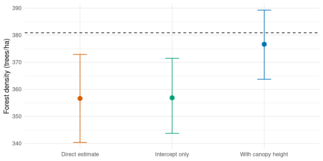
The known forest density is 380.9 trees/ha. All three estimates use the same 151 sampled plots. Only the model with canopy height uses predictor information across the forest. We compare their estimates and intervals with the known density below.
ggplot(comparison, aes(method, estimate, color = method)) +
  geom_hline(yintercept = true_forest_density, linetype = "dashed") +
  geom_errorbar(aes(ymin = lower, ymax = upper), width = 0.15) +
  geom_point(size = 3) +
  scale_color_manual(values = c("Direct estimate" = "#D55E00",
                                "Intercept only" = "#009E73",
                                "With canopy height" = "#0072B2")) +
  labs(x = NULL, y = "Forest density (trees/ha)") +
  theme_minimal() +
  theme(legend.position = "none")
Here the intercept-only estimate is close to the direct estimate. Adding canopy height brings the forest estimate closer to truth and gives a somewhat narrower interval. The canopy-height model accounts for differences in the predictor distribution between sampled plots and the forest grid.
A design-based confidence interval is interpreted through repeated sampling from the same forest. The model interval assigns 95% posterior probability to the stated range for forest density, conditional on the observations, model, and priors. Their widths need not agree, and adding a predictor does not guarantee a narrower interval.
Estimate stand densities
The same predictions also give density estimates for each of the 249 stands. Some cells cross stand boundaries, so we use the area of each cell within each stand as its weight. A cell contributes the same predicted density draw to every stand it overlaps.
We read the overlap table constructed in the data article. In standSummary(), unit identifies the prediction cell, group identifies the stand, and represented_area gives its area within that stand. The function averages densities within each stand for every posterior draw.
cell_stand_areas <- read_csv("data/cell_stand_areas.csv")

stand_predictions <- standSummary(
  predictions,
  data = cell_stand_areas,
  unit = prediction_id,
  group = stand_id,
  represented_area = area_ha,
  summary = "samples"
)

stand_estimates <- summary(stand_predictions) |>
  transmute(stand_id = unit, estimate = mean, lower = q2_5, upper = q97_5)
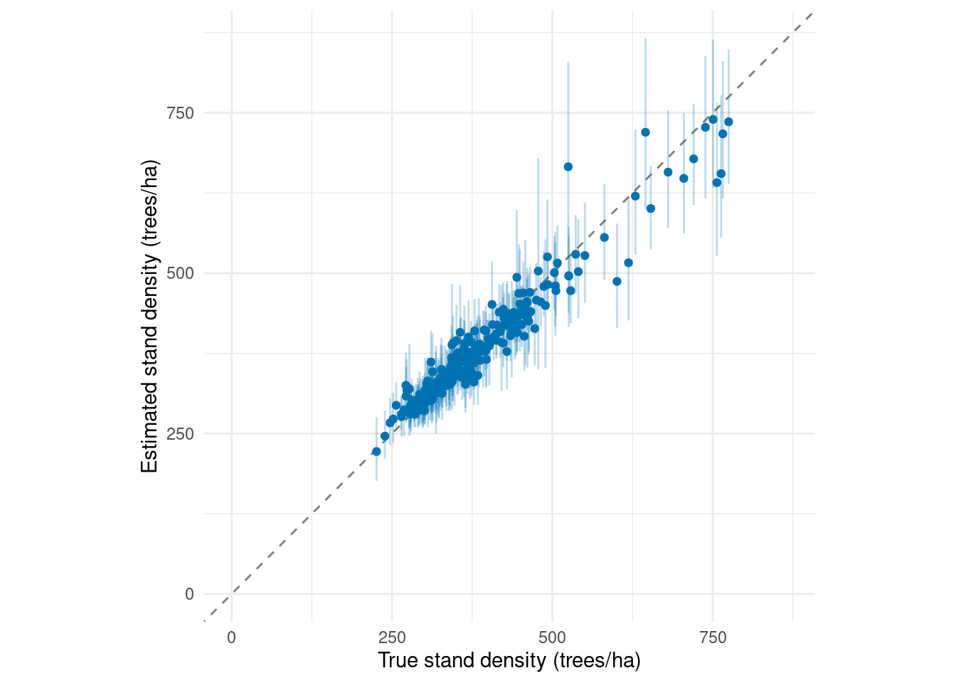
We calculate true stand densities from the simulated cell counts using the same overlap areas, then compare estimates and their 95% posterior predictive intervals with truth. The dashed line marks equality.
stand_truth <- cell_stand_areas |>
  left_join(
    prediction |> transmute(prediction_id = plot_id, density = count / area),
    by = "prediction_id"
  ) |>
  group_by(stand_id) |>
  summarise(truth = weighted.mean(density, area_ha), .groups = "drop")

stand_estimates <- stand_estimates |>
  left_join(stand_truth, by = "stand_id")

stand_limits <- range(0, stand_estimates$truth, stand_estimates$lower,
                       stand_estimates$upper)

ggplot(stand_estimates, aes(truth, estimate)) +
  geom_abline(intercept = 0, slope = 1, linetype = "dashed", color = "grey50") +
  geom_errorbar(aes(ymin = lower, ymax = upper), width = 0,
                 color = "#0072B2", alpha = 0.25) +
  geom_point(color = "#0072B2", size = 1.5) +
  coord_equal(xlim = stand_limits, ylim = stand_limits) +
  labs(x = "True stand density (trees/ha)",
       y = "Estimated stand density (trees/ha)") +
  theme_minimal()
The model gives estimates for stands with and without sampled plots because canopy height is available across the forest. Each interval summarizes the aggregated predictive draws for that stand.
The next article fits species composition to describe how a known total is allocated among species.
References
Spitta, Arthur, Andrew O. Finley, Christoph Gollob, Ralf Kraßnitzer, Tim Ritter, Andreas Tockner, and Arne Nothdurft. 2026.
“Evaluating LiDAR Data Sources, Predictor Resolution, and Spatial Random Effects in Bayesian Change-of-Support Models for Forest Inventory.” arXiv Preprint arXiv:2610.06476.
https://doi.org/10.48550/arXiv.2610.06476.