Composition describes each species’ share of the trees. Using the shared simulated forest, we relate the allocation of trees among pine, oak, and birch to canopy height. We fit a composition-only model, compare its coefficients with their generating values, and estimate forest-wide species proportions conditional on known total counts in the prediction cells.
Example data
Download the plot-sampling data (ZIP)
The introductory plot-sampling articles use this same archive. Extract it and use the folder containing data/ as your R working directory.
Read the data
We use the same 151 sampled plots and 4,812 prediction cells as the magnitude article. The tables contain simulated total counts and species-by-DBH counts, along with plot or cell area in hectares and standardized canopy height x. We read both tables and sum the DBH-class counts within each species.
library(magComp)
library(tidyverse)

set.seed(1)

plots <- read_csv("data/plots.csv")

prediction <- read_csv("data/prediction.csv")

species_order <- c("pine", "oak", "birch")

# Columns such as pine:10-20 contain species-by-DBH counts.
trees <- plots |>
  select(plot_id, area, x, contains(":")) |>
  pivot_longer(contains(":"), names_to = c("species", "dbh_class"),
               names_sep = ":", values_to = "count") |>
  group_by(plot_id, area, x, species) |>
  summarise(count = sum(count), .groups = "drop") |>
  mutate(species = factor(species, levels = species_order)) |>
  arrange(plot_id, species)

trees |>
  filter(plot_id == 1) |>
  knitr::kable(digits = 3)
| 1 |
0.126 |
-0.811 |
pine |
20 |
| 1 |
0.126 |
-0.811 |
oak |
15 |
| 1 |
0.126 |
-0.811 |
birch |
20 |
The resulting trees table has one row per plot and species, including species with zero counts. The predictor x is p95 standardized using the plots’ mean and standard deviation; the same scaling was applied to the prediction cells in the data article.
Model species composition
For plot , let be its total tree count, the count of species , and that species’ probability. The probabilities sum to one, and the model allocates the known total using
We use the species sequence pine, oak, birch. The model first allocates trees to pine, then allocates some of the remaining trees to oak; birch receives the rest. Let be the pine probability and the oak probability among trees that are not pine. The default probit link gives
where and are the intercept and slope for allocation step . The standard normal distribution function , implemented by pnorm() in R, converts the linear expression to a probability. The overall species probabilities are
For example, if pine receives 50% of the trees and oak receives 60% of those remaining, the overall proportions are 50% pine, 30% oak, and 20% birch. Birch has no separate coefficient row. Species have no natural order; the chosen sequence defines the allocation steps and the interpretation of their coefficients.
Fit and examine parameter estimates
magCompData() obtains each plot’s total by summing its species counts. We set magnitude = NULL to fit composition alone. The formula ~ x supplies an intercept and canopy-height slope for each allocation step, and ordered = FALSE specifies unordered species categories without smoothing across them.
dat <- magCompData(
  trees,
  unit = plot_id, category = species, tree_count = count,
  ordered = FALSE, design = fixedArea(area)
)

fit <- magComp(
  dat,
  magnitude = NULL,
  composition = ~ x,
  control = magCompControl(
    n_samples = 2000,
    n_burn = 1000,
    n_chains = 3,
    n_cores = 3,
    chain_seeds = 1:3,
    verbose = FALSE
  )
)
We use default independent Normal coefficient priors and starting values. Each of three MCMC chains runs for 2,000 iterations and discards the first 1,000, leaving 3,000 draws for parameter summaries. Plot area is not needed to estimate species probabilities, but supplying it allows conditional counts to be expressed as densities.
We compare the estimated coefficients with the values used in the data article. Named values match each parameter’s printed index.
true_alpha <- c("pine:(Intercept)" = 0, "pine:x" = 0.5,
                "oak:(Intercept)" = -0.5, "oak:x" = -0.5)

parameter_summary <- summary(fit)
parameter_summary$truth <- true_alpha[parameter_summary$index]

parameter_summary |>
  select(symbol, truth, mean, q2_5, q97_5, rhat, ess) |>
  knitr::kable(
    digits = 3,
    col.names = c("Parameter", "Truth", "Mean", "2.5%", "97.5%", "R-hat", "ESS")
  )
| alpha[0,pine] |
0.0 |
0.010 |
-0.024 |
0.042 |
1.000 |
1151.637 |
| alpha[x,pine] |
0.5 |
0.490 |
0.455 |
0.525 |
1.000 |
804.009 |
| alpha[0,oak] |
-0.5 |
-0.505 |
-0.560 |
-0.452 |
1.005 |
731.858 |
| alpha[x,oak] |
-0.5 |
-0.496 |
-0.543 |
-0.448 |
1.005 |
662.682 |
The labels alpha[0,pine] and alpha[x,pine] denote pine’s intercept and slope. Applying pnorm() to an intercept gives the conditional probability at average plot p95. A positive slope increases that probability as canopy height increases; for oak, this describes its share among trees remaining after pine. The slopes are on the probit scale, so they are not constant percentage-point changes in species proportions.
The mean and 2.5% and 97.5% columns give posterior estimates and 95% credible intervals. All four generating values fall within these intervals. R-hat values near one indicate agreement among chains; ESS is the effective sample size after accounting for dependence among iterations.
Predict forest composition
Species probabilities can be predicted from canopy height alone. To estimate each species’ share of all trees in the forest, we also need the abundance in each cell. Here we supply the simulated cell totals as known inputs using total_count = "count". The cell’s species counts remain unknown to the model and are used below to calculate truth.
For each retained parameter draw, target = "observation" allocates each cell’s total among the species with a multinomial draw. We request density, which divides the resulting species counts by cell area, and use 100 draws per chain for prediction.
predictions <- predict(
  fit,
  prediction |> select(plot_id, x, area, count),
  total_count = "count",
  type = "density",
  target = "observation",
  n_draws = 100,
  summary = "samples"
)

# Prediction cell x species x retained draw x chain.
dim(predictions$density)
#> [1] 4812    3  100    3
The array contains 4,812 cells, three species, 100 draws, and three chains. Each allocation sums to its supplied cell total. Uncertainty comes from the coefficients and species allocation, conditional on those fixed totals.
We pass these draws to standSummary() to calculate forest composition. Within each draw, it multiplies species densities by represented cell areas, sums over cells, and divides each species’ total by the total across species. Thus, cells with more trees contribute more to the forest’s species proportions. Omitting group produces one forest-wide summary.
forest_predictions <- standSummary(
  predictions,
  data = prediction,
  unit = plot_id,
  represented_area = area,
  type = "proportion",
  summary = "samples"
)

forest_summary <- summary(forest_predictions)
forest_summary
#> magComp standSummary summary (target = 'observation')
#> Counts condition on supplied totals.
#> Proportions condition on a positive total.
#>  unit   quantity category   mean       sd   q2_5    q50  q97_5 n_draws
#>   all proportion     pine 0.4226 0.005224 0.4117 0.4229 0.4329     300
#>   all proportion      oak 0.2964 0.004837 0.2870 0.2962 0.3053     300
#>   all proportion    birch 0.2811 0.005494 0.2705 0.2809 0.2920     300
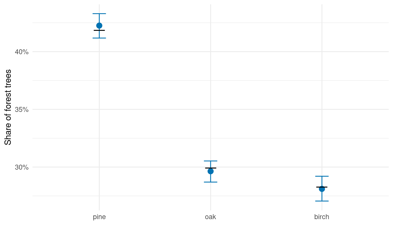
The mean column gives each species’ estimated share of forest trees. The q2_5 and q97_5 columns bound its 95% posterior predictive interval. Species proportions sum to one in every draw, as do their posterior means; their separate interval endpoints need not sum to one.
Compare with truth
We calculate true proportions by summing the simulated species-by-DBH counts across prediction cells and DBH classes, then dividing each species’ total by the forest total. These are the same cell-area weights used above, since multiplying a cell’s density by its area returns its count.
We show the estimated proportions and their intervals alongside the known forest proportions.
The estimates closely match the known forest composition, and all three true proportions fall within their intervals. These intervals condition on known cell totals. When those totals must also be estimated, we combine magnitude and composition to predict both abundance and its allocation. The next article does this for DBH classes across all species, followed by a species-by-DBH model. Both carry uncertainty from magnitude and composition into forest and stand summaries.