A manager may want a stand’s diameter distribution without distinguishing species. We use the shared simulated forest, sum tree counts over species within each diameter at breast height (DBH) class, and fit a magnitude model together with a single ordered composition model. We then compare predicted forest and stand DBH distributions with the known distributions in that population.
The magnitude article estimates overall tree density, while the composition article estimates species shares conditional on known totals. Here magnitude supplies the total and composition allocates it among DBH classes. Together they produce a one-dimensional stand table in trees per hectare.
Example data
Download the plot-sampling data (ZIP)
The introductory plot-sampling articles use this same archive. Extract it and use the folder containing data/ as your R working directory.
Sum counts within DBH classes
We read the 151 sampled plots and 4,812 prediction cells. Both tables contain species-by-DBH counts, area in hectares, and canopy-height predictor x, standardized using the plots’ mean and standard deviation. We sum the plot counts over species so the data supplied to the model have one row per plot and DBH class, including zero counts.
library(magComp)
library(tidyverse)

set.seed(1)

plots <- read_csv("data/plots.csv")

prediction <- read_csv("data/prediction.csv")

dbh_classes <- c("10-20", "20-30", "30-40", "40-50", "50+")

trees <- plots |>
  select(plot_id, area, x, contains(":")) |>
  pivot_longer(contains(":"), names_to = c("species", "dbh_class"),
               names_sep = ":", values_to = "count") |>
  group_by(plot_id, area, x, dbh_class) |>
  summarise(count = sum(count), .groups = "drop") |>
  mutate(dbh_class = ordered(dbh_class, levels = dbh_classes)) |>
  arrange(plot_id, dbh_class)

trees |>
  filter(plot_id == 1) |>
  knitr::kable(digits = 3)
| 1 |
0.126 |
-0.811 |
10-20 |
25 |
| 1 |
0.126 |
-0.811 |
20-30 |
15 |
| 1 |
0.126 |
-0.811 |
30-40 |
9 |
| 1 |
0.126 |
-0.811 |
40-50 |
4 |
| 1 |
0.126 |
-0.811 |
50+ |
2 |
Each class includes its lower bound and excludes its upper bound; 50+ contains trees at least 50 cm in diameter. Species no longer enters the model. Summing the five counts still gives each plot’s original total.
Model total counts and DBH allocation
For plot , let be its total count, its sampled area in hectares, and its expected density in trees/ha. The magnitude model is
where the negative-binomial distribution has mean and size . The composition model allocates this total among the five DBH classes,
Here counts trees in class , and is its probability. As in the composition article, allocation proceeds sequentially using a probit model. For each of the first four classes,
is the probability of entering class among trees not yet allocated to a smaller class. The final class receives the remainder. Each step has its own intercept and canopy-height slope. The resulting expected density in class is , and the five densities sum to .
Fit and check the model
We supply DBH as the only category and give both model components a canopy-height predictor. magCompData() obtains total counts by summing the DBH-class counts within each plot.
dat <- magCompData(
  trees,
  unit = plot_id, category = dbh_class, tree_count = count,
  design = fixedArea(area)
)

fit <- magComp(
  dat,
  magnitude = ~ x,
  composition = ~ x,
  control = magCompControl(
    n_samples = 2000,
    n_burn = 1000,
    n_chains = 3,
    n_cores = 3,
    chain_seeds = 1:3,
    verbose = FALSE
  )
)
We use default priors and automatic starting values, estimating negative-binomial size along with the regression coefficients. Each chain runs for 2,000 iterations and discards the first 1,000. The ordered factor sets the allocation sequence; it does not automatically smooth coefficients across DBH classes. Smoothing can be added through magCompSmooth().
We inspect posterior estimates, 95% credible intervals, R-hat, and effective sample size (ESS) with summary(). R-hat values near one indicate agreement among chains; ESS accounts for dependence among successive draws.
parameter_summary <- summary(fit)

parameter_summary |>
  select(symbol, mean, q2_5, q97_5, rhat, ess) |>
  knitr::kable(
    digits = 3,
    col.names = c("Parameter", "Mean", "2.5%", "97.5%", "R-hat", "ESS")
  )
| beta[0] |
5.857 |
5.825 |
5.888 |
1.000 |
2793.771 |
| beta[x] |
-0.186 |
-0.217 |
-0.155 |
1.001 |
2318.698 |
| r_M |
66.394 |
37.877 |
116.976 |
1.002 |
575.741 |
| alpha[0,10-20] |
-0.531 |
-0.564 |
-0.496 |
1.000 |
1041.488 |
| alpha[x,10-20] |
-0.346 |
-0.377 |
-0.314 |
1.000 |
1028.748 |
| alpha[0,20-30] |
-0.165 |
-0.205 |
-0.125 |
1.001 |
1198.109 |
| alpha[x,20-30] |
-0.379 |
-0.420 |
-0.339 |
1.001 |
1105.471 |
| alpha[0,30-40] |
0.168 |
0.117 |
0.219 |
1.004 |
1271.296 |
| alpha[x,30-40] |
-0.236 |
-0.294 |
-0.178 |
1.001 |
1161.417 |
| alpha[0,40-50] |
0.483 |
0.397 |
0.574 |
1.000 |
891.955 |
| alpha[x,40-50] |
-0.136 |
-0.235 |
-0.037 |
1.002 |
823.180 |
The chains agree closely for these parameters. We now assess the quantities of interest, the DBH-class densities.
Predict the forest DBH distribution
At each prediction cell, target = "observation" first draws a total count from the magnitude model and then allocates it among DBH classes. type = "density" divides those counts by cell area. We use 100 retained draws from each chain, giving 300 joint predictions across the forest.
predictions <- predict(
  fit,
  prediction |> select(plot_id, x, area),
  type = "density",
  target = "observation",
  n_draws = 100,
  summary = "samples"
)

# Prediction cell x DBH class x retained draw x chain.
dim(predictions$density)
#> [1] 4812    5  100    3
We pass these draws to standSummary(), which averages densities within each draw using the cells’ areas as weights. Omitting group produces a forest-wide summary. The intervals include uncertainty about total counts and their allocation among DBH classes.
forest_predictions <- standSummary(
  predictions,
  data = prediction,
  unit = plot_id,
  represented_area = area,
  summary = "samples"
)

forest_summary <- summary(forest_predictions)
To calculate truth, we sum the simulated prediction-cell counts over species within each DBH class, just as we did for the plots. Forest density is the class count summed across cells divided by their combined area.
cell_counts <- prediction |>
  select(plot_id, area, contains(":")) |>
  pivot_longer(contains(":"), names_to = c("species", "dbh_class"),
               names_sep = ":", values_to = "count") |>
  group_by(plot_id, area, dbh_class) |>
  summarise(count = sum(count), .groups = "drop")

forest_truth <- cell_counts |>
  group_by(dbh_class) |>
  summarise(truth = sum(count) / sum(area), .groups = "drop")

forest_comparison <- forest_summary |>
  as_tibble() |>
  rename(dbh_class = category) |>
  left_join(forest_truth, by = "dbh_class") |>
  mutate(dbh_class = ordered(dbh_class, levels = dbh_classes))

forest_comparison |>
  select(dbh_class, truth, mean, q2_5, q97_5) |>
  knitr::kable(digits = 2,
               col.names = c("DBH class", "Truth", "Mean", "2.5%", "97.5%"))
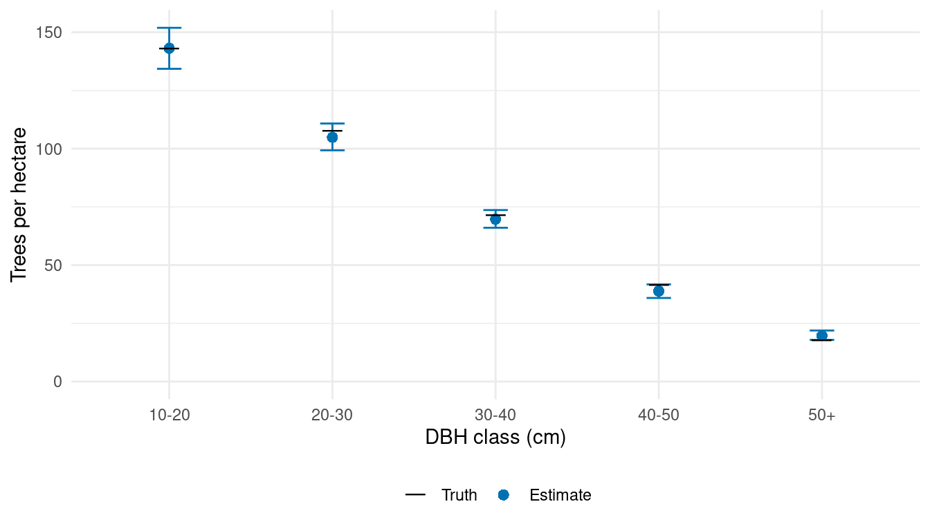
| 10-20 |
142.93 |
143.11 |
134.30 |
151.91 |
| 20-30 |
107.50 |
104.86 |
99.29 |
110.81 |
| 30-40 |
71.48 |
69.71 |
66.04 |
73.64 |
| 40-50 |
41.31 |
38.86 |
35.88 |
41.73 |
| 50+ |
17.68 |
19.70 |
17.89 |
21.90 |
We compare the estimated DBH distribution with the realized population distribution. Each point estimates trees per hectare in one DBH class.
ggplot(forest_comparison, aes(dbh_class, mean)) +
  geom_errorbar(aes(ymin = q2_5, ymax = q97_5), width = 0.15,
                color = "#0072B2") +
  geom_point(aes(shape = "Estimate"), color = "#0072B2", size = 2.5) +
  geom_point(aes(y = truth, shape = "Truth"), size = 6) +
  scale_shape_manual(values = c("Truth" = 95, "Estimate" = 16),
                     breaks = c("Truth", "Estimate"), name = NULL) +
  scale_y_continuous(limits = c(0, NA)) +
  labs(x = "DBH class (cm)", y = "Trees per hectare") +
  theme_minimal() +
  theme(legend.position = "bottom")
The estimated distribution follows the population’s decline in density across increasing DBH classes. Four of the five intervals contain the true forest densities. The 50+ class is overestimated by about 2 trees/ha, with truth just below its interval.
Compare stand DBH distributions
The same predictions give stand-level estimates. We read the cell–stand overlap areas prepared in the data article and supply group = stand_id. Cells crossing stand boundaries contribute the same density draw to each stand, weighted by their area within that stand.
cell_stand_areas <- read_csv("data/cell_stand_areas.csv")

stand_predictions <- standSummary(
  predictions,
  data = cell_stand_areas,
  unit = prediction_id,
  group = stand_id,
  represented_area = area_ha,
  summary = "samples"
)

stand_summary <- summary(stand_predictions)
We calculate true stand densities from the simulated cell counts using those same overlap areas, then match them to the estimates by stand and DBH class.
stand_truth <- cell_counts |>
  mutate(density = count / area) |>
  inner_join(cell_stand_areas, by = c("plot_id" = "prediction_id"),
             relationship = "many-to-many") |>
  group_by(stand_id, dbh_class) |>
  summarise(truth = weighted.mean(density, area_ha), .groups = "drop")

stand_comparison <- stand_summary |>
  as_tibble() |>
  rename(stand_id = unit, dbh_class = category) |>
  left_join(stand_truth, by = c("stand_id", "dbh_class")) |>
  mutate(dbh_class = ordered(dbh_class, levels = dbh_classes))
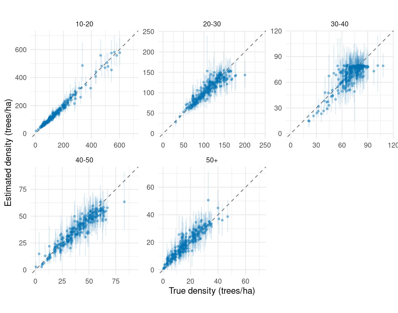
Each panel compares predicted and true density in one DBH class across all 249 stands. Points near the dashed line indicate close agreement; the vertical bars show uncertainty in each stand estimate.
# Give both axes the same upper limit within each DBH panel.
stand_limits <- stand_comparison |>
  group_by(dbh_class) |>
  summarise(limit = max(truth, mean, q97_5), .groups = "drop")

ggplot(stand_comparison, aes(truth, mean)) +
  geom_blank(data = stand_limits, aes(x = limit, y = limit)) +
  geom_abline(intercept = 0, slope = 1, linetype = "dashed", color = "grey50") +
  geom_errorbar(aes(ymin = q2_5, ymax = q97_5), width = 0,
                color = "#0072B2", alpha = 0.12) +
  geom_point(color = "#0072B2", size = 0.9, alpha = 0.4) +
  facet_wrap(~ dbh_class, ncol = 3, scales = "free") +
  scale_x_continuous(limits = c(0, NA)) +
  scale_y_continuous(limits = c(0, NA)) +
  labs(x = "True density (trees/ha)", y = "Estimated density (trees/ha)") +
  theme_minimal() +
  theme(aspect.ratio = 1)
The stand comparisons show differences that a forest average can conceal. Agreement is strongest in the smallest DBH class; individual stands show more scatter relative to their densities in the middle and larger classes.
When species also matters
We have fitted DBH counts summed over species. If species-specific estimates are also needed, the next article fits the species-by-DBH model. Its predictions can also produce a DBH distribution across species by summing species densities within each posterior draw, before calculating means and intervals. This is the DBH margin in Equation (28) of Finley et al. (2026).
That approach retains species information during fitting. It targets the same DBH densities as this article, but the estimates need not be identical because the fitted models differ.
References
Finley, Andrew O., Malcolm S. Itter, Arthur Spitta, and Arne Nothdurft. 2026. “A Bayesian Magnitude-Composition Model for Tree-Size Distributions and Stand-Tables.”