Function for prediction at new locations using NNGP models.

The function predict collects posterior predictive samples for a set of new locations given an object of class NNGP.

Usage

# S3 method for class 'NNGP'
predict(object, X.0, coords.0, sub.sample,
        n.omp.threads = 1, verbose=TRUE, n.report=100, ...)

Arguments

object

an object of class NNGP.

X.0

the design matrix for prediction locations. An intercept should be provided in the first column if one is specified in sp.obj model.

coords.0

the spatial coordinates corresponding to X.0.

sub.sample

an optional list that specifies the samples to included in the composition sampling a non-Conjugate model. Valid tags are start, end, and thin. Given the value associated with the tags, the sample subset is selected using seq(as.integer(start), as.integer(end), by=as.integer(thin)). The default values are start=floor(0.5*n.samples), end=n.samples and thin=1.

n.omp.threads

a positive integer indicating the number of threads to use for SMP parallel processing. The package must be compiled for OpenMP support. For most Intel-based machines, we recommend setting n.omp.threads up to the number of hyperthreaded cores. Note, n.omp.threads > 1 might not work on some systems.

verbose

if TRUE, model specification and progress of the sampler is printed to the screen. Otherwise, nothing is printed to the screen.

n.report

the interval to report sampling progress.

...

currently no additional arguments.

Value

An object of class predict.NNGP which is a list comprising:

p.y.0

a matrix that holds the response variable posterior predictive samples where rows are locations corresponding to coords.0 and columns are samples.

p.w.0

a matrix that holds the random effect posterior predictive samples where rows are locations corresponding to coords.0 and columns are samples. This is only returned if the input class has method = "latent".

run.time

execution time reported using proc.time().

References

Datta, A., S. Banerjee, A.O. Finley, and A.E. Gelfand. (2016) Hierarchical Nearest-Neighbor Gaussian process models for large geostatistical datasets. Journal of the American Statistical Association, doi:10.1080/01621459.2015.1044091 .

Finley, A.O., A. Datta, B.D. Cook, D.C. Morton, H.E. Andersen, and S. Banerjee. (2019) Efficient algorithms for Bayesian Nearest Neighbor Gaussian Processes. Jurnal of Computational and Graphical Statistics, doi:10.1080/10618600.2018.1537924 .

Author

Andrew O. Finley finleya@msu.edu,
Abhirup Datta abhidatta@jhu.edu,
Sudipto Banerjee sudipto@ucla.edu

Examples

rmvn <- function(n, mu=0, V = matrix(1)){
  p <- length(mu)
  if(any(is.na(match(dim(V),p))))
    stop("Dimension problem!")
  D <- chol(V)
  t(matrix(rnorm(n*p), ncol=p)%*%D + rep(mu,rep(n,p)))
}

##Make some data
set.seed(1)
n <- 100
coords <- cbind(runif(n,0,1), runif(n,0,1))

x <- cbind(1, rnorm(n))

B <- as.matrix(c(1,5))

sigma.sq <- 5
tau.sq <- 1
phi <- 3/0.5

D <- as.matrix(dist(coords))
R <- exp(-phi*D)
w <- rmvn(1, rep(0,n), sigma.sq*R)
y <- rnorm(n, x%*%B + w, sqrt(tau.sq))

ho <- sample(1:n, 50)

y.ho <- y[ho]
x.ho <- x[ho,,drop=FALSE]
w.ho <- w[ho]
coords.ho <- coords[ho,]

y <- y[-ho]
x <- x[-ho,,drop=FALSE]
w <- w[-ho,,drop=FALSE]
coords <- coords[-ho,]

##Fit a Response, Latent, and Conjugate NNGP model
n.samples <- 500

starting <- list("phi"=phi, "sigma.sq"=5, "tau.sq"=1)

tuning <- list("phi"=0.5, "sigma.sq"=0.5, "tau.sq"=0.5)

priors <- list("phi.Unif"=c(3/1, 3/0.01), "sigma.sq.IG"=c(2, 5), "tau.sq.IG"=c(2, 1))

cov.model <- "exponential"

n.report <- 500

##Latent
m.s <- spNNGP(y~x-1, coords=coords, starting=starting, method="latent", n.neighbors=10,
              tuning=tuning, priors=priors, cov.model=cov.model,
              n.samples=n.samples, n.omp.threads=1, n.report=n.report)
#> ----------------------------------------
#> 	Building the neighbor list
#> ----------------------------------------
#> ----------------------------------------
#> Building the neighbors of neighbors list
#> ----------------------------------------
#> ----------------------------------------
#> 	Model description
#> ----------------------------------------
#> NNGP Latent model fit with 50 observations.
#> 
#> Number of covariates 2 (including intercept if specified).
#> 
#> Using the exponential spatial correlation model.
#> 
#> Using 10 nearest neighbors.
#> 
#> Number of MCMC samples 500.
#> 
#> Priors and hyperpriors:
#> 	beta flat.
#> 	sigma.sq IG hyperpriors shape=2.00000 and scale=5.00000
#> 	tau.sq IG hyperpriors shape=2.00000 and scale=1.00000
#> 	phi Unif hyperpriors a=3.00000 and b=300.00000
#> 
#> Source compiled with OpenMP support and model fit using 1 thread(s).
#> ----------------------------------------
#> 		Sampling
#> ----------------------------------------
#> Sampled: 500 of 500, 100.00%
#> Report interval Metrop. Acceptance rate: 69.80%
#> Overall Metrop. Acceptance rate: 69.80%
#> -------------------------------------------------

p.s <- predict(m.s, X.0 = x.ho, coords.0 = coords.ho, n.omp.threads=1)
#> ----------------------------------------
#> 	Prediction description
#> ----------------------------------------
#> NNGP Latent model fit with 50 observations.
#> 
#> Number of covariates 2 (including intercept if specified).
#> 
#> Using the exponential spatial correlation model.
#> 
#> Using 10 nearest neighbors.
#> 
#> Number of MCMC samples 500.
#> 
#> Predicting at 50 locations.
#> 
#> 
#> Source compiled with OpenMP support and model fit using 1 threads.
#> -------------------------------------------------
#> 		Predicting
#> -------------------------------------------------
#> Location: 50 of 50, 100.00%

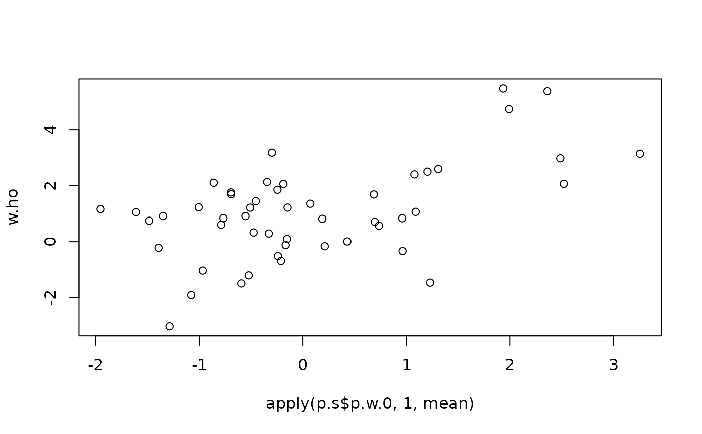
plot(apply(p.s$p.w.0, 1, mean), w.ho)

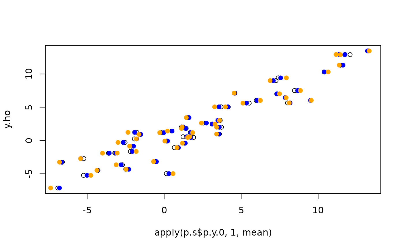
plot(apply(p.s$p.y.0, 1, mean), y.ho)

##Response
m.r <- spNNGP(y~x-1, coords=coords, starting=starting, method="response", n.neighbors=10,
              tuning=tuning, priors=priors, cov.model=cov.model,
              n.samples=n.samples, n.omp.threads=1, n.report=n.report)
#> ----------------------------------------
#> 	Building the neighbor list
#> ----------------------------------------
#> ----------------------------------------
#> 	Model description
#> ----------------------------------------
#> NNGP Response model fit with 50 observations.
#> 
#> Number of covariates 2 (including intercept if specified).
#> 
#> Using the exponential spatial correlation model.
#> 
#> Using 10 nearest neighbors.
#> 
#> Number of MCMC samples 500.
#> 
#> Priors and hyperpriors:
#> 	beta flat.
#> 	sigma.sq IG hyperpriors shape=2.00000 and scale=5.00000
#> 	tau.sq IG hyperpriors shape=2.00000 and scale=1.00000
#> 	phi Unif hyperpriors a=3.00000 and b=300.00000
#> 
#> Source compiled with OpenMP support and model fit using 1 thread(s).
#> ----------------------------------------
#> 		Sampling
#> ----------------------------------------
#> Sampled: 500 of 500, 100.00%
#> Report interval Metrop. Acceptance rate: 37.40%
#> Overall Metrop. Acceptance rate: 37.40%
#> -------------------------------------------------

p.r <- predict(m.r, X.0 = x.ho, coords.0 = coords.ho, n.omp.threads=1)
#> ----------------------------------------
#> 	Prediction description
#> ----------------------------------------
#> NNGP Response model fit with 50 observations.
#> 
#> Number of covariates 2 (including intercept if specified).
#> 
#> Using the exponential spatial correlation model.
#> 
#> Using 10 nearest neighbors.
#> 
#> Number of MCMC samples 500.
#> 
#> Predicting at 50 locations.
#> 
#> 
#> Source compiled with OpenMP support and model fit using 1 threads.
#> -------------------------------------------------
#> 		Predicting
#> -------------------------------------------------
#> Location: 50 of 50, 100.00%

points(apply(p.r$p.y.0, 1, mean), y.ho, pch=19, col="blue")

##Conjugate
theta.alpha <- c(phi, tau.sq/sigma.sq)
names(theta.alpha) <- c("phi", "alpha")

m.c <- spConjNNGP(y~x-1, coords=coords, n.neighbors=10,
                  theta.alpha=theta.alpha, sigma.sq.IG=c(2, sigma.sq),
                  cov.model=cov.model, n.omp.threads=1)
#> ----------------------------------------
#> 	Model description
#> ----------------------------------------
#> NNGP Conjugate model fit with 50 observations.
#> 
#> Number of covariates 2 (including intercept if specified).
#> 
#> Using the exponential spatial correlation model.
#> 
#> Using 10 nearest neighbors.
#> 
#> Source compiled with OpenMP support and model fit using 1 thread(s).
#> ------------
#> Priors and hyperpriors:
#> 	beta flat.
#> 	sigma.sq IG hyperpriors shape=2.00000 and scale=5.00000
#> ------------
#> 	Estimation for parameter set(s)
#> Set phi=6.00000 and alpha=0.20000

p.c <- predict(m.c, X.0 = x.ho, coords.0 = coords.ho, n.omp.threads=1)
#> ----------------------------------------
#> 	Model description
#> ----------------------------------------
#> NNGP Conjugate model fit with 50 observations.
#> 
#> Number of covariates 2 (including intercept if specified).
#> 
#> Using the exponential spatial correlation model.
#> 
#> Using 10 nearest neighbors.
#> 
#> Source compiled with OpenMP support and model fit using 1 thread(s).
#> ------------
#> Priors and hyperpriors:
#> 	beta flat.
#> 	sigma.sq IG hyperpriors shape=2.00000 and scale=5.00000
#> ------------
#> Predicting at 50 locations.
#> ------------
#> 	Estimation for parameter set(s)
#> Set phi=6.00000 and alpha=0.20000

points(p.c$y.0.hat, y.ho, pch=19, col="orange")