
Continuous space-time NNGP models with stLMM
Point observations, joint grid prediction, and areal summaries
Source:vignettes/a05-space-time-nngp.qmd
1 Overview
This vignette fits a continuous space-time model for point observations using an NNGP latent process. In a small-area estimation setting, this is a unit-level model: the model is fit to observations at their point locations and time indices, then posterior predictions are made over a chosen areal space-time support and aggregated to produce small-area estimates.
This builds on the point observations with areal space-time effects article. There, point observations were mapped to a county-year latent support before fitting. Here, the latent process remains continuous in space and indexed by year. We then create county and state summaries after fitting by predicting on a space-time grid over Washington counties. The grid below is modest for readability. In applied analyses, you would usually use a denser grid, remotely sensed pixels, or another set of integration points with scientifically meaningful weights.
2 Model
For observation \(i\) at location \(\mathbf{s}_i = (s_{i1}, s_{i2})^\top\) and time index \(t_i\), the model is
\[ y_i = \beta_0 + x_i\beta_1 + w(\mathbf{s}_i,t_i) + \epsilon_i,\qquad \epsilon_i \sim N(0,\tau^2). \]
The continuous space-time process is
\[ \mathbf{w} = \{w(\mathbf{s}_1,t_1),\ldots,w(\mathbf{s}_n,t_n)\}^\top \sim N(\mathbf{0}, \sigma^2 \mathbf{R}(a,c,\alpha,\beta,\gamma,\delta)). \]
We simulate the dataset using the two-spatial-dimensional exponential special case of the nonseparable correlation function in Equation (12) of Gneiting (2002). This is the same covariance as Equation (6.1) of Datta, Banerjee, Finley, Hamm, et al. (2016).
\[ R_{ij}(a,c,\alpha,\beta,\gamma,\delta) = \{1+a |t_i-t_j|^{2\alpha}\}^{-(\delta + d/2)} \exp\left[ -\frac{c \|\mathbf{s}_i-\mathbf{s}_j\|^{2\gamma}}{\{1+a |t_i-t_j|^{2\alpha}\}^{\beta\gamma}} \right]. \]
The spatial dimension is \(d = 2\). This example follows the Datta et al. special case by fixing alpha = 1, gamma = 0.5, and delta = 0, and estimating a, c, and the interaction parameter beta. Here a controls temporal decay at the same location, c controls spatial decay at the same time, and beta controls departure from separability by allowing the effective spatial range to change with temporal lag. When beta = 0, the model reduces to the separable product of an exponential spatial correlation and a Cauchy-like temporal correlation.
The fitted model uses nngp() as a nearest-neighbor approximation to this full Gaussian process covariance. The approximation keeps the same covariance function but avoids dense full-GP covariance calculations that become expensive for larger datasets; see Datta, Banerjee, Finley, and Gelfand (2016) and Finley et al. (2019) for NNGP model and computation details. Space-time NNGP models and related space-time latent Gaussian process models are developed and applied in Datta, Banerjee, Finley, Hamm, et al. (2016) and May and Finley (2025).
3 Simulated point observations
We use Washington counties to define the simulation domain and the later aggregation supports. The stunitco geometries are already stored in a projected coordinate reference system for these examples. Their coordinates are in meters, which would make spatial decay parameters hard to interpret. We divide the projected coordinates by 1000 and fit the model in kilometers. With this scaling, spatial ranges and prior bounds can be expressed directly in kilometers.
Code
data(stunitco, package = "stLMM")

wa_counties <- stunitco[stunitco$STATECD == 53, ]
wa_counties$county <- wa_counties$COUNTYNM

year <- 1:8
n_year <- sample(55:75, length(year), replace = TRUE)
wa_union <- sf::st_union(sf::st_geometry(wa_counties))
wa_crs <- sf::st_crs(wa_counties)

plot_dat <- data.frame()

for(j in seq_along(year)){
  year_sf <- sf::st_sf(
    geometry = sf::st_sample(wa_union, size = n_year[j])
  )
  year_sf <- sf::st_join(
    year_sf,
    wa_counties[, "county"],
    join = sf::st_within,
    left = FALSE
  )
  year_coord <- sf::st_coordinates(year_sf)
  year_dat <- data.frame(
    year = year[j],
    county = year_sf$county,
    x_m = year_coord[, 1],
    y_m = year_coord[, 2],
    x_km = year_coord[, 1] / 1000,
    y_km = year_coord[, 2] / 1000
  )
  plot_dat <- rbind(plot_dat, year_dat)
}

plot_dat$obs_id <- seq_len(nrow(plot_dat))
plot_dat <- plot_dat[order(plot_dat$year, plot_dat$obs_id), ]
rownames(plot_dat) <- NULL

x_trend <- (plot_dat$x_km - mean(plot_dat$x_km)) -
  0.4 * (plot_dat$y_km - mean(plot_dat$y_km))
x_mean <- mean(x_trend)
x_sd <- stats::sd(x_trend)
plot_dat$x <- (x_trend - x_mean) / x_sd

beta <- c(0.5, 1)
sigma_sq <- 1
range_correlation <- 0.05
spatial_range_km <- 250
temporal_range_years <- 5
a <- (1 / range_correlation - 1) / temporal_range_years^2
c <- -log(range_correlation) / spatial_range_km
alpha <- 1
beta_gneiting <- 0.5
gamma <- 0.5
delta <- 0
tau_sq <- 0.05

C <- gneiting_cov(
  coords = plot_dat[, c("x_km", "y_km")],
  time = plot_dat$year,
  sigma_sq = sigma_sq,
  a = a,
  c = c,
  alpha = alpha,
  beta = beta_gneiting,
  gamma = gamma,
  delta = delta
)

plot_dat$w_true <- rmvnorm(mean = rep(0, nrow(plot_dat)), Sigma = C)

mu <- beta[1] + beta[2] * plot_dat$x + plot_dat$w_true
epsilon <- rnorm(nrow(plot_dat), sd = sqrt(tau_sq))
plot_dat$y <- mu + epsilon
The faceted map shows the simulated point observations within Washington counties. The model is fit to the points; the counties are used later as reporting units.
Show plotting code
point_sf <- sf::st_as_sf(
  plot_dat,
  coords = c("x_m", "y_m"),
  crs = wa_crs
)

ggplot() +
  geom_sf(
    data = wa_counties,
    fill = "grey95",
    color = "white",
    linewidth = 0.1
  ) +
  geom_sf(
    data = point_sf,
    aes(color = y),
    size = 0.8,
    alpha = 0.75
  ) +
  scale_color_gradientn(colors = stlmm_palette()) +
  facet_wrap(~ year, ncol = 4) +
  labs(color = "response")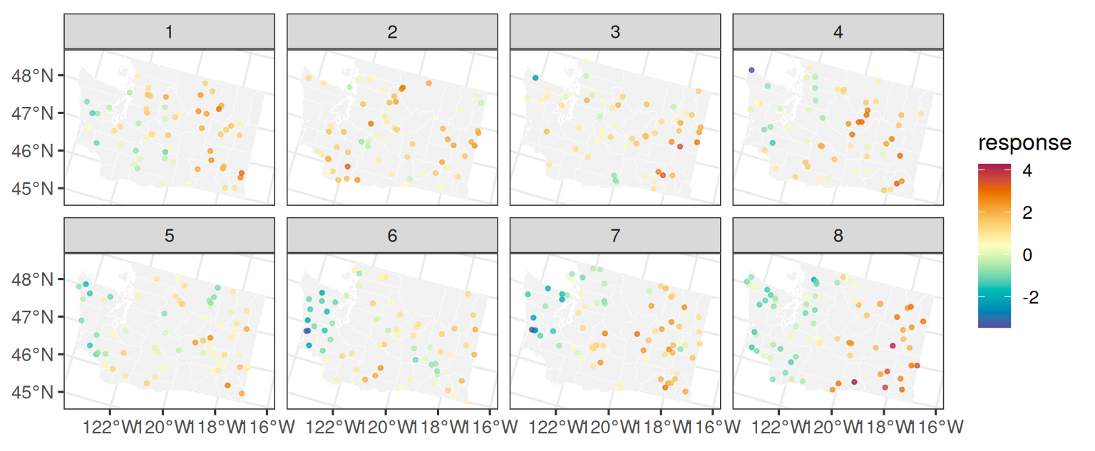
4 Fit
The simulated dataset was generated from a full Gaussian process with the gneiting covariance model. The fitted model below uses nngp() as an approximation to that full Gaussian process. The formula uses the point-level covariate x and a continuous space-time NNGP over projected spatial coordinates in kilometers, x_km and y_km, and the time index year.
The last coordinate in nngp() is treated as time for space-time covariance models such as cov_model = "gneiting". Thus nngp(x_coord, y_coord, time, cov_model = "gneiting") is not the same as putting the time coordinate first.
The covariance model has six Gneiting parameters. To keep this example identifiable and close to the Datta et al. special case, we fix alpha = 1, gamma = 0.5, and delta = 0, and estimate the temporal scale a, spatial decay c, and interaction parameter beta. We set prior bounds by first choosing interpretable same-time spatial ranges in kilometers and same-location temporal ranges in years, then converting those ranges to bounds for c and a. These are marginal range interpretations along the spatial and temporal axes. Away from those axes, the full space-time correlation surface also depends on beta.
Code
prior_correlation <- 0.05
spatial_prior_range_km <- c(80, 600)
temporal_prior_range_years <- c(3, 8)

c_prior <- -log(prior_correlation) / rev(spatial_prior_range_km)
a_prior <- (1 / prior_correlation - 1) / rev(temporal_prior_range_years)^2

fit <- stLMM(
  y ~ x + nngp(x_km, y_km, year, m = 15, cov_model = "gneiting", ordering = "coord"),
  data = plot_dat,
  starting = list(
    nngp_1 = list(
      alpha = fixed(1),
      gamma = fixed(0.5),
      delta = fixed(0)
    )
  ),
  priors = list(
    resid = list(tau_sq = half_t(df = 3, scale = 0.5)),
    nngp_1 = list(
      sigma_sq = half_t(df = 3, scale = 1),
      a = uniform(a_prior[1], a_prior[2]),
      c = uniform(c_prior[1], c_prior[2]),
      beta = uniform(0.05, 0.95)
    )
  ),
  n_samples = 400,
  verbose = FALSE
)

summary(fit)
stLMM summary
formula: y ~ x + nngp(x_km, y_km, year, m = 15, cov_model = "gneiting", ordering = "coord")
observations: 508
posterior draws: 400
family: gaussian
fixed effects: 2
grouped random-effect coefficients: 0
process terms: 1
residual variance: global tau_sq
beta:
mean sd q2.5 q50.0 q97.5
(Intercept) 0.8147 0.1527 0.5046 0.8176 1.1250
x 0.8287 0.1197 0.6076 0.8320 1.0534
tau_sq:
mean sd q2.5 q50.0 q97.5
value 0.0241 0.0207 6e-04 0.0184 0.0697
sigma_sq:
mean sd q2.5 q50.0 q97.5
nngp_1_sigma_sq 1.0677 0.1059 0.8883 1.0583 1.2654
theta:
mean sd q2.5 q50.0 q97.5
nngp_1_a 1.3794 0.3596 0.7951 1.4423 1.9566
nngp_1_c 0.0145 0.0021 0.0105 0.0145 0.0181
nngp_1_alpha 1.0000 0.0000 1.0000 1.0000 1.0000
nngp_1_beta 0.3115 0.1439 0.1191 0.3009 0.7097
nngp_1_gamma 0.5000 0.0000 0.5000 0.5000 0.5000
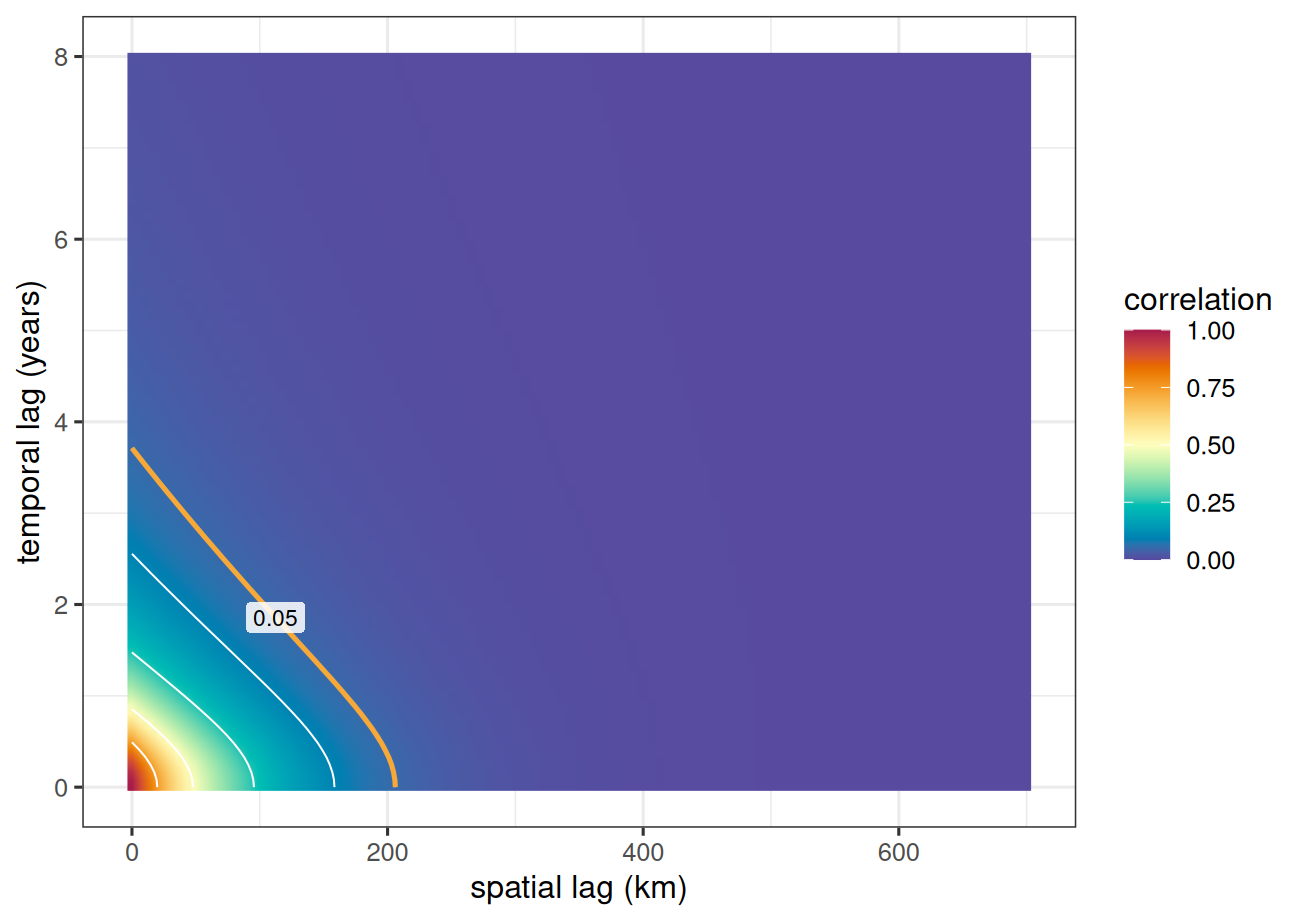
nngp_1_delta 0.0000 0.0000 0.0000 0.0000 0.0000The posterior mean covariance parameters imply the following correlation surface over spatial lag and temporal lag. This plot is a useful way to interpret the fitted covariance because it shows how spatial and temporal separation combine. The contour lines mark correlation levels; the 0.05 contour is a visual reference for an effective space-time range.
Show plotting code
fit_draws <- as_samples(fit, metadata = FALSE)
theta_cols <- c(
  "nngp_1_a",
  "nngp_1_c",
  "nngp_1_alpha",
  "nngp_1_beta",
  "nngp_1_gamma",
  "nngp_1_delta"
)
theta_mean <- colMeans(fit_draws[, theta_cols, drop = FALSE])
surface_theta <- setNames(
  as.numeric(theta_mean),
  c("a", "c", "alpha", "beta", "gamma", "delta")
)

spatial_lag <- seq(0, 700, length.out = 100)
temporal_lag <- seq(0, 8, length.out = 100)
surface <- outer(
  spatial_lag,
  temporal_lag,
  Vectorize(function(h, u){
    scale <- 1 + surface_theta["a"] * abs(u)^(2 * surface_theta["alpha"])
    scale^(-(surface_theta["delta"] + 1)) *
      exp(-surface_theta["c"] * h^(2 * surface_theta["gamma"]) /
            scale^(surface_theta["beta"] * surface_theta["gamma"]))
  })
)

surface_dat <- expand.grid(
  spatial_lag = spatial_lag,
  temporal_lag = temporal_lag
)
surface_dat$correlation <- as.vector(surface)

contour_breaks <- c(0.05, 0.10, 0.25, 0.50, 0.75)
contour_lines <- contourLines(
  x = spatial_lag,
  y = temporal_lag,
  z = surface,
  levels = 0.05
)
contour_labels <- data.frame(
  spatial_lag = numeric(0),
  temporal_lag = numeric(0),
  label = character(0)
)

for(j in seq_along(contour_lines)){
  line_midpoint <- ceiling(length(contour_lines[[j]]$x) / 2)
  contour_labels <- rbind(
    contour_labels,
    data.frame(
      spatial_lag = contour_lines[[j]]$x[line_midpoint],
      temporal_lag = contour_lines[[j]]$y[line_midpoint],
      label = format(contour_lines[[j]]$level, nsmall = 2)
    )
  )
}

ggplot(surface_dat, aes(spatial_lag, temporal_lag, z = correlation)) +
  geom_raster(aes(fill = correlation), interpolate = TRUE) +
  geom_contour(
    breaks = contour_breaks,
    color = "white",
    linewidth = 0.35
  ) +
  geom_contour(
    breaks = 0.05,
    color = stlmm_color("contrast"),
    linewidth = 0.9
  ) +
  geom_label(
    data = contour_labels,
    aes(spatial_lag, temporal_lag, label = label),
    inherit.aes = FALSE,
    size = 3,
    label.size = 0,
    fill = "white",
    alpha = 0.85
  ) +
  scale_fill_gradientn(colors = stlmm_palette(), limits = c(0, 1)) +
  labs(
    x = "spatial lag (km)",
    y = "temporal lag (years)",
    fill = "correlation"
  )
5 Recover observed space-time effects
The NNGP latent process is integrated out during fitting. Calling recover() draws the fitted space-time random effects conditional on the retained posterior samples. We recover these effects before prediction because prediction from a process model uses posterior draws of the latent process as part of the fitted model state.
stLMM recovery
  formula: y ~ x + nngp(x_km, y_km, year, m = 15, cov_model = "gneiting", ordering = "coord")
  observations: 508
  recovered draws: 126
  recovered process terms: nngp_1
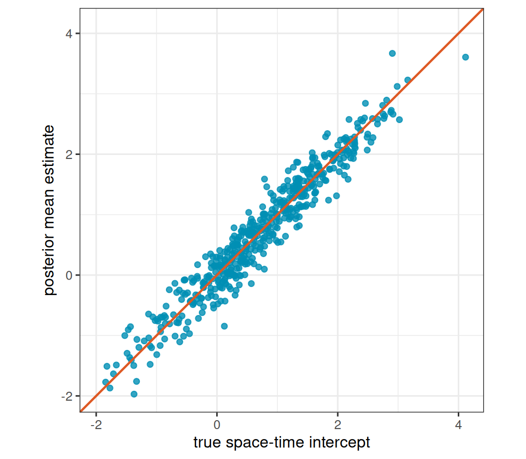
As in the previous NNGP examples, the data identify the combined space-time intercept, \(\beta_0 + w(\mathbf{s}_i,t_i)\), more directly than the split between the global intercept and the average level of one realized process. For that reason, the diagnostic below compares the recovered combined intercept to its simulated value.
Show plotting code
rec_draws <- as_samples(rec, include_w = TRUE, metadata = FALSE)
w_cols <- paste0("w_nngp_1_", seq_len(nrow(plot_dat)))
w_hat <- colMeans(rec_draws[, w_cols, drop = FALSE])
beta_0_hat <- mean(rec_draws[["(Intercept)"]])

recovery_dat <- data.frame(
  truth = beta[1] + plot_dat$w_true,
  estimate = beta_0_hat + w_hat
)
recovery_lim <- range(recovery_dat$truth, recovery_dat$estimate)

ggplot(recovery_dat, aes(truth, estimate)) +
  geom_point(
    color = stlmm_color("primary"),
    size = 1.7,
    alpha = 0.8
  ) +
  geom_abline(
    intercept = 0,
    slope = 1,
    color = stlmm_color("secondary"),
    linewidth = 0.8
  ) +
  coord_equal(
    xlim = recovery_lim,
    ylim = recovery_lim
  ) +
  labs(
    x = "true space-time intercept",
    y = "posterior mean estimate"
  )
6 Space-time prediction grid
For county and state summaries, we create a modest regular prediction grid over the union of Washington counties and cross it with the eight time points. This is a simplified version of the integration grid one would use for small-area estimation. Each grid point is assigned to its containing county for aggregation. The grid-point covariate is computed from the same coordinate-based rule used for the observed sites, so predictions are made under the same data-generating relationship.
Code
county_area <- as.numeric(sf::st_area(wa_counties))
names(county_area) <- wa_counties$county

grid_geometry <- sf::st_make_grid(wa_union, n = c(35, 24), what = "centers")
grid_sf <- sf::st_sf(geometry = grid_geometry)
grid_sf <- grid_sf[lengths(sf::st_within(grid_sf, wa_union)) > 0, ]
grid_sf <- sf::st_join(
  grid_sf,
  wa_counties[, "county"],
  join = sf::st_within,
  left = FALSE
)
grid_coord <- sf::st_coordinates(grid_sf)

space_grid <- data.frame(
  county = grid_sf$county,
  x_m = grid_coord[, 1],
  y_m = grid_coord[, 2],
  x_km = grid_coord[, 1] / 1000,
  y_km = grid_coord[, 2] / 1000
)
grid_x_trend <- (space_grid$x_km - mean(plot_dat$x_km)) -
  0.4 * (space_grid$y_km - mean(plot_dat$y_km))
space_grid$x <- (grid_x_trend - x_mean) / x_sd

pred_grid <- data.frame()
for(yy in year){
  year_grid <- space_grid
  year_grid$year <- yy
  pred_grid <- rbind(pred_grid, year_grid)
}
pred_grid <- pred_grid[order(pred_grid$county, pred_grid$year), ]

grid_count <- table(space_grid$county)
pred_grid$weight <- county_area[pred_grid$county] / as.numeric(grid_count[pred_grid$county])
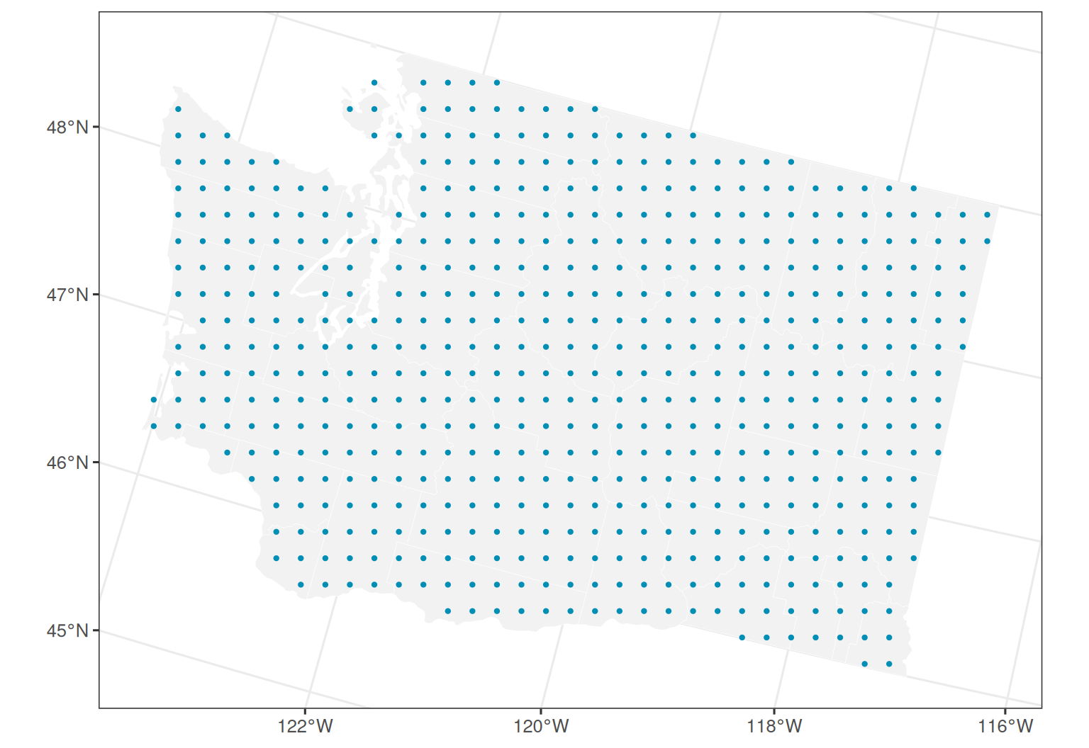
The map below shows the spatial grid used for prediction and aggregation. In an applied analysis, these grid points would usually be replaced by a denser grid, remotely sensed pixels, or another integration support chosen for the target summaries.
Show plotting code
7 Joint prediction and aggregation
We use joint prediction because county and state summaries are functions of many predicted values. With joint = TRUE, posterior dependence among prediction points is propagated into the aggregated summaries. The vecchia joint method avoids forming a dense covariance over all new prediction locations and is the better choice for larger prediction grids. This prediction approach is related to Vecchia-style prediction methods for Gaussian processes; see Katzfuss and Guinness (2021).
For space-time NNGP prediction, st_scale affects nearest-neighbor ranking for new prediction locations by multiplying the time coordinate before neighbor search. It does not change the covariance function after neighbors are selected. Because spatial coordinates are in kilometers and time is in years, st_scale = 75 treats a one-year temporal gap as roughly comparable to 75 kilometers for neighbor ranking.
Code
stLMM prediction
  mean samples: 126 draws x 4536 rows
  newdata: TRUE
  joint: TRUE
  y samples: not simulated
  process samples: nngp_1
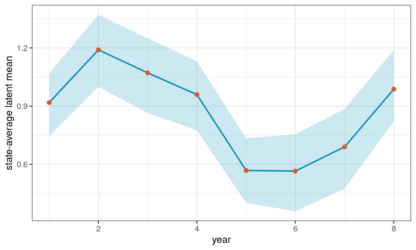
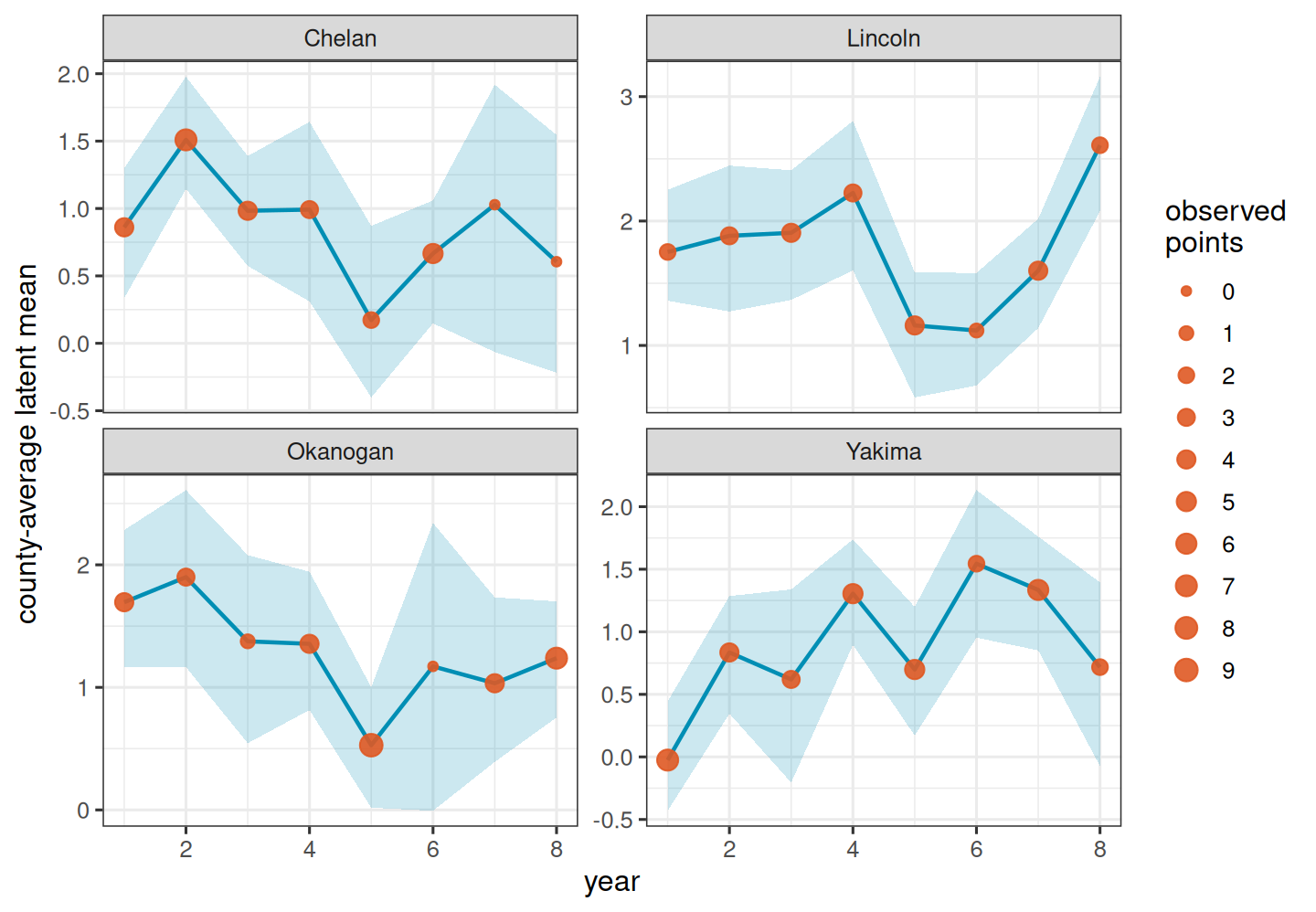
The prediction object contains posterior samples of the latent mean, \(\mu\), at each grid point and year. County-year summaries average those samples over grid points inside each county. State-year summaries average over all grid points using weights proportional to county area in this simplified example.
Code
pred_mu <- as_samples(pred, sample = "mu", metadata = FALSE)
county_year <- unique(pred_grid[, c("county", "year")])
county_year <- county_year[order(county_year$county, county_year$year), ]
county_samples <- matrix(
  NA_real_,
  nrow = nrow(pred_mu),
  ncol = nrow(county_year)
)

for(j in seq_len(nrow(county_year))){
  ii <- which(
    pred_grid$county == county_year$county[j] &
      pred_grid$year == county_year$year[j]
  )
  county_samples[, j] <- rowMeans(pred_mu[, ii, drop = FALSE])
}

county_summary <- data.frame(
  county = county_year$county,
  year = county_year$year,
  mean = colMeans(county_samples),
  lower = NA_real_,
  upper = NA_real_
)

for(j in seq_len(ncol(county_samples))){
  county_summary$lower[j] <- quantile(county_samples[, j], probs = 0.025)
  county_summary$upper[j] <- quantile(county_samples[, j], probs = 0.975)
}

state_samples <- matrix(
  NA_real_,
  nrow = nrow(pred_mu),
  ncol = length(year),
  dimnames = list(NULL, year)
)

for(j in seq_along(year)){
  ii <- which(pred_grid$year == year[j])
  ww <- pred_grid$weight[ii] / sum(pred_grid$weight[ii])
  state_samples[, j] <- as.numeric(as.matrix(pred_mu[, ii, drop = FALSE]) %*% ww)
}

state_summary <- data.frame(
  year = year,
  mean = colMeans(state_samples),
  lower = NA_real_,
  upper = NA_real_
)

for(j in seq_len(ncol(state_samples))){
  state_summary$lower[j] <- quantile(state_samples[, j], probs = 0.025)
  state_summary$upper[j] <- quantile(state_samples[, j], probs = 0.975)
}
Before looking at the aggregate time series, it is useful to check the grid-level predictions. The faceted map below colors each prediction grid point by its posterior mean \(\mu\) for that year.
Show plotting code
pred_point_dat <- pred_grid
pred_point_dat$mu_mean <- colMeans(pred_mu)

pred_point_sf <- sf::st_as_sf(
  pred_point_dat,
  coords = c("x_m", "y_m"),
  crs = wa_crs
)

ggplot() +
  geom_sf(
    data = wa_counties,
    fill = "grey95",
    color = "white",
    linewidth = 0.1
  ) +
  geom_sf(
    data = pred_point_sf,
    aes(color = mu_mean),
    size = 0.55
  ) +
  scale_color_gradientn(colors = stlmm_palette()) +
  facet_wrap(~ year, ncol = 4) +
  labs(color = "posterior\nmean")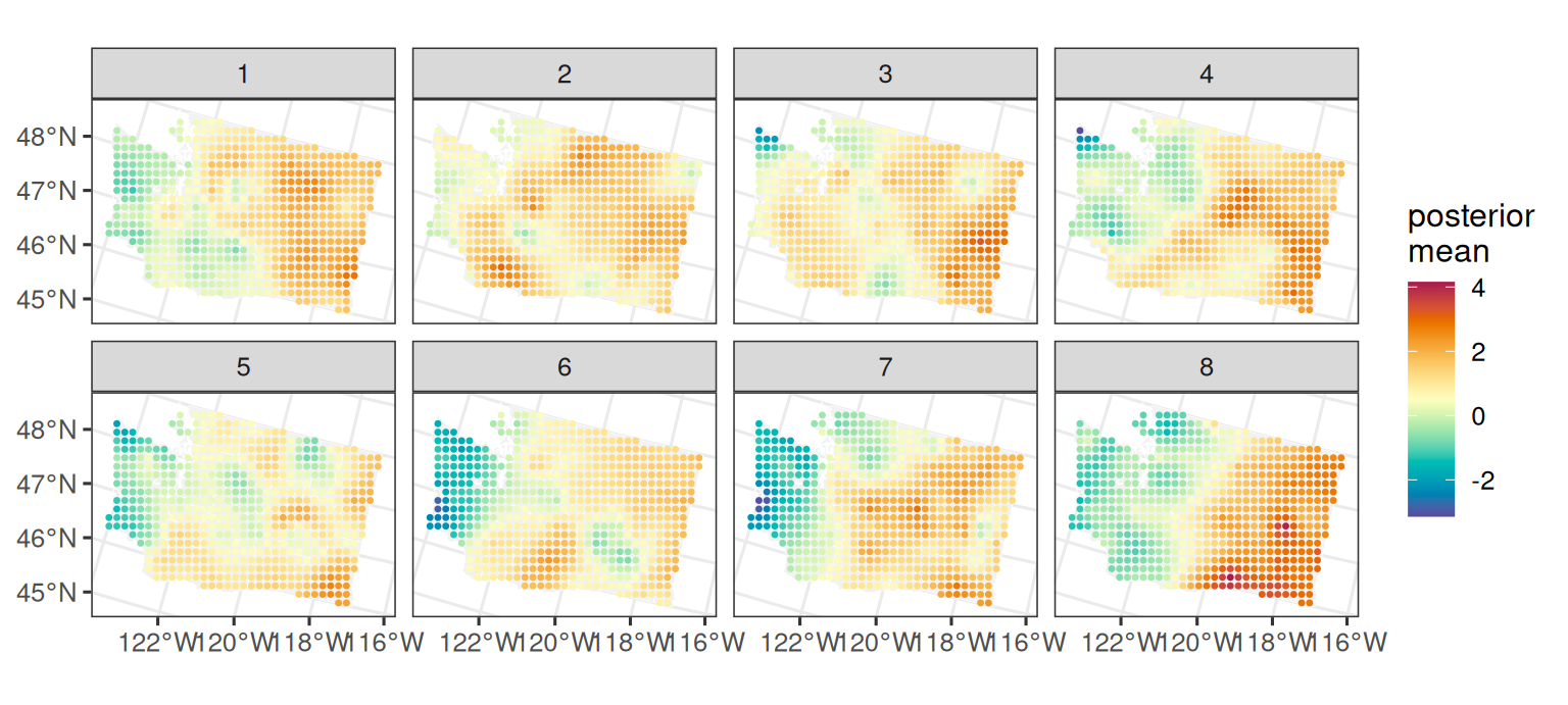
The state time series aggregates the grid-level posterior samples over Washington for each year. The ribbon shows pointwise 95% posterior intervals for the state-average latent mean.
Show plotting code
ggplot(state_summary, aes(year, mean)) +
  geom_ribbon(
    aes(ymin = lower, ymax = upper),
    fill = stlmm_color("primary"),
    alpha = 0.2
  ) +
  geom_line(
    color = stlmm_color("primary"),
    linewidth = 0.8
  ) +
  geom_point(
    color = stlmm_color("secondary"),
    size = 2
  ) +
  labs(
    x = "year",
    y = "state-average latent mean"
  )
8 County time series
County-specific time series are useful for checking how prediction uncertainty changes when a county has few or no observations at a given time. The figure below marks the number of observed point responses in each county-year, so the reader can compare posterior uncertainty with the amount of local information.
Show plotting code
obs_count <- aggregate(
  y ~ county + year,
  data = plot_dat,
  FUN = length
)
names(obs_count)[names(obs_count) == "y"] <- "n_obs"

county_rank <- data.frame(county = sort(unique(plot_dat$county)))
county_rank$n_obs <- 0
for(j in seq_len(nrow(county_rank))){
  county_rank$n_obs[j] <- sum(plot_dat$county == county_rank$county[j])
}
county_rank <- county_rank[order(-county_rank$n_obs), ]
selected_county <- head(county_rank$county, 4)

series_dat <- county_summary[county_summary$county %in% selected_county, ]
series_dat$n_obs <- 0
for(j in seq_len(nrow(series_dat))){
  matched <- obs_count$county == series_dat$county[j] &
    obs_count$year == series_dat$year[j]
  if(any(matched))
    series_dat$n_obs[j] <- obs_count$n_obs[matched][1]
}

ggplot(series_dat, aes(year, mean)) +
  geom_ribbon(
    aes(ymin = lower, ymax = upper),
    fill = stlmm_color("primary"),
    alpha = 0.2
  ) +
  geom_line(
    color = stlmm_color("primary"),
    linewidth = 0.8
  ) +
  geom_point(
    aes(size = n_obs),
    color = stlmm_color("secondary"),
    alpha = 0.9
  ) +
  facet_wrap(~ county, scales = "free_y", ncol = 2) +
  scale_size_continuous(
    range = c(1.5, 4),
    breaks = seq(0, max(series_dat$n_obs))
  ) +
  labs(
    x = "year",
    y = "county-average latent mean",
    size = "observed\npoints"
  )
9 What this example illustrates
The model is continuous in space and indexed by time because the latent process uses point coordinates and the observed time index directly. County and state estimates are not latent CAR effects. They are posterior summaries created by predicting over a chosen support and then aggregating those prediction samples.
The prediction grid in this vignette is simple for readability. A full small-area estimation workflow would replace it with a denser spatial grid, pixels from auxiliary data products, or another integration support, then aggregate posterior samples using the desired area or population weights.
Joint prediction is most useful when the target is an aggregate, contrast, exceedance area, or other function of multiple prediction points. Marginal prediction with joint = FALSE can be faster for maps of posterior means or pointwise intervals, but it does not preserve posterior dependence among new prediction locations.