
Washington county biomass SAE overview
Data, estimands, and the model tour
Source:vignettes/wa-county-biomass-overview.qmd
1 Purpose
This article opens a Washington county biomass small-area estimation series. The series is motivated by USDA Forest Service Forest Inventory and Analysis (FIA) data, the national forest inventory of the United States (USDA Forest Service Forest Inventory and Analysis Program 2026; Bechtold and Patterson 2005). It uses a single prepared data bundle to show how stLMM can fit related area-level and unit-level models for county-level forest inventory inference over time.
The series focuses on stLMM model structures and software workflows. It therefore uses a deliberately simplified working target that keeps the area-response and unit-response articles aimed at the same quantity. The model tour below defines that quantity and distinguishes it from FIA’s formal forestland biomass estimands.
The articles use modest sampler settings and compact prediction grids so the examples are runnable. Production analyses should use longer chains, broader diagnostics, sensitivity checks, and application-specific validation.
Each article in the series is reproducible from its Quarto source or extracted R code. Those source links appear near the top of each article. The shared Washington biomass data bundle is linked from each article and is the only data download needed for the series.
2 Running the Articles
Download the Washington biomass data bundle and unzip it before running an article locally. The archive expands to a directory named wa_data containing the county geometry, direct-estimate table, FIA plot table, and compact prediction grids used across the series.
Run each Quarto source file or extracted R script from the directory that contains wa_data. With that layout, the article setup uses data_dir <- "wa_data", and all data inputs are read with paths such as file.path(data_dir, "wa_unit_plots.csv").
For example, a local working directory for an extracted article should look like this:
my-wa-article-run/
  wa-direct-car-time.R
  article-utils.R
  article-cache.R
  wa_data/
    wa_counties.rds
    wa_direct_estimates.csv
    wa_unit_plots.csv
    wa_unit_prediction_grid_5km.csv
    wa_unit_prediction_grid_10km.csv
The articles do not read raw FIA tables or TCC rasters. They read only the prepared files in wa_data.
3 Model Tour
3.1 Working Target
The main series estimates the county-year mean of one plot-level response. For plot row \(j\), \(y_j\) is the agb_live_mg_ha column.
This variable is live aboveground tree biomass density in Mg/ha computed from live trees on FIA forest conditions. Plot rows with no live forest-condition biomass are recorded as zero. For county \(a\) and year \(t\), the series target is the average value of the agb_live_mg_ha response over the county-year support used for prediction or aggregation. We denote that county-year target by \(\theta_{a,t}\). This target is intentionally simple: it is the mean of agb_live_mg_ha on the analysis support, not a formal FIA forestland ratio estimator.
3.2 Area-Response Models
Area-response articles model county-year direct estimates of this target. The direct estimate is the sample mean of agb_live_mg_ha among observed FIA plot rows,
\[ \hat{y}_{a,t} = \frac{1}{n_{a,t}}\sum_{j \in S_{a,t}} y_j, \]
where \(S_{a,t}\) is the set of FIA plot rows observed in county \(a\) and year \(t\), and \(n_{a,t}\) is the number of rows in that set. Throughout the area-response articles, \(\hat{y}\) denotes a direct estimate and \(\theta\) denotes the latent county-year biomass mean that the direct estimate is estimating. The estimated sampling variance used in these tutorial examples is the usual sample variance of \(y_j\) divided by \(n_{a,t}\), with the direct-estimate articles documenting the model-ready treatment of zero and missing variance estimates.
The area-response models are Fay-Herriot-style small-area models (Fay and Herriot 1979): the direct estimate is noisy, the sampling variance tells the model how noisy it is, and spatial or space-time random effects borrow strength across neighboring counties and nearby years. The series starts with CAR-time smoothing of direct estimates, then adds county mean TCC as a remote-sensing covariate, scaled direct-estimate variances, and a spatially varying TCC effect. County-years with only one FIA plot are retained in the county-year support, but they are not treated as direct estimates because no sampling variance can be estimated from one plot.
3.3 Unit-Response Models
Unit-response articles model the same agb_live_mg_ha response at FIA plot locations and then aggregate predictions over a county-year grid using
\[ \theta_{a,t} = \operatorname{avg}_{g \in U_{a,t}} \tilde{y}_g, \]
where \(U_{a,t}\) is the set of prediction-grid rows assigned to county \(a\) and year \(t\), and \(\tilde{y}_g\) is a model-based prediction for grid row \(g\). The grid provides a common support for summarizing unit-response predictions at the county-year scale.
The unit-response models are BHF-style unit-level SAE models (Battese et al. 1988). The series starts with BHF models that use row-level TCC, county random effects, and a shared year effect, then moves to two-stage county-time CAR models, FIA-unit-specific residual variances, and continuous space-time prediction.
Because agb_live_mg_ha has a point mass at zero and a long positive tail, the unit-response sequence also includes two-stage models. For equivalence with the area-response direct estimates in this series, the binary stage is agb_live_mg_ha > 0, and the continuous stage models positive agb_live_mg_ha. Predictions combine the two stages draw by draw, following the hurdle-style product used in related forest-biomass applications (Finley et al. 2011; May and Finley 2025).
3.4 FIA Design Deferred
FIA forested status and proportion_forested describe forestland support, not merely whether agb_live_mg_ha is positive. A model that uses those variables as the first stage moves the estimand toward an FIA forestland-support target. That is scientifically important, but it is different from the series target above.
Formal FIA estimators use condition proportions, stratification and nonresponse adjustments, domain definitions such as forestland, and ratio estimators for per-acre quantities (Bechtold and Patterson 2005; Stanke et al. 2020). Model-based inference that remains faithful to complex sampling designs is an active research area, especially when the population units have spatial or multivariate dependence (Banerjee 2024). The series concludes with a Colville National Forest capstone that is closer to that target: it estimates biomass on forested land within a user-defined spatial extent in Washington by modeling forestland occurrence and positive biomass before aggregating over the target area (Finley et al. 2011; May and Finley 2025).
4 Data Bundle
Show data-reading code
data_dir <- "wa_data"

wa_counties <- read_rds(file.path(data_dir, "wa_counties.rds"))
unit_plots <- read_csv(file.path(data_dir, "wa_unit_plots.csv"), show_col_types = FALSE)
direct_estimates <- read_csv(file.path(data_dir, "wa_direct_estimates.csv"), show_col_types = FALSE)
grid_5km <- read_csv(file.path(data_dir, "wa_unit_prediction_grid_5km.csv"), show_col_types = FALSE)
grid_10km <- read_csv(file.path(data_dir, "wa_unit_prediction_grid_10km.csv"), show_col_types = FALSE)
manifest <- read_csv(file.path(data_dir, "DATA_MANIFEST.csv"), show_col_types = FALSE)

unit_plots <- unit_plots |>
  mutate(
    forested = as.logical(forested),
    county_fips = as.character(county_fips)
  )

direct_estimates <- direct_estimates |>
  mutate(county_fips = as.character(county_fips))

grid_5km <- grid_5km |>
  mutate(county_fips = as.character(county_fips))
The data pack is built from raw FIA tables and annual USDA Forest Service Tree Canopy Cover rasters (USDA Forest Service 2026). Plot-level and grid-level TCC values are sampled from the annual TCC raster at each location. County-year mean TCC summarizes the annual TCC raster within each county.
Show data-pack summary code
data_pack_summary <- tibble(
  quantity = c(
    "counties",
    "FIA units",
    "direct-estimate years",
    "unit plot rows",
    "direct-estimate rows",
    "model-ready direct-estimate rows",
    "single-plot rows retained but excluded",
    "direct-estimate rows using variance floor",
    "5 km prediction-grid rows",
    "10 km prediction-grid rows",
    "plot rows dropped for missing TCC"
  ),
  value = c(
    nrow(wa_counties),
    n_distinct(unit_plots$fia_unit),
    n_distinct(direct_estimates$year),
    nrow(unit_plots),
    nrow(direct_estimates),
    manifest_value("direct_estimate_model_rows"),
    manifest_value("direct_estimate_single_plot_excluded_rows"),
    manifest_value("direct_estimate_variance_floor_rows"),
    manifest_value("prediction_grid_5km_full_rows"),
    nrow(grid_10km),
    manifest_value("unit_plot_dropped_missing_tcc_rows")
  )
) |>
  mutate(value = fmt_int(as.numeric(value)))

show_table(data_pack_summary, caption = "Washington county biomass article data bundle.")| quantity | value |
|---|---|
| counties | 39 |
| FIA units | 5 |
| direct-estimate years | 10 |
| unit plot rows | 6,935 |
| direct-estimate rows | 390 |
| model-ready direct-estimate rows | 315 |
| single-plot rows retained but excluded | 15 |
| direct-estimate rows using variance floor | 60 |
| 5 km prediction-grid rows | 70,340 |
| 10 km prediction-grid rows | 17,620 |
| plot rows dropped for missing TCC | 3 |
5 Data Characteristics
Show plot summary table code
plot_status_summary <- unit_plots |>
  mutate(status = if_else(forested, "forested", "nonforested")) |>
  count(status, name = "plot_rows") |>
  mutate(percent = 100 * plot_rows / sum(plot_rows))

fia_unit_summary <- unit_plots |>
  mutate(status = if_else(forested, "forested", "nonforested")) |>
  count(fia_unit, fia_unit_name, status, name = "plot_rows") |>
  pivot_wider(names_from = status, values_from = plot_rows, values_fill = 0) |>
  mutate(
    total = forested + nonforested,
    forested_percent = 100 * forested / total
  ) |>
  arrange(fia_unit)

show_table(
  plot_status_summary |>
    mutate(
      plot_rows = fmt_int(plot_rows),
      percent = fmt_num(percent, 1)
    ),
  caption = "Forested and nonforested FIA plot rows."
)| status | plot_rows | percent |
|---|---|---|
| forested | 4,239 | 61.1 |
| nonforested | 2,696 | 38.9 |
Show plot summary table code
| fia_unit | fia_unit_name | forested | nonforested | total | forested_percent |
|---|---|---|---|---|---|
| 5 | Puget Sound | 762 | 379 | 1,141 | 66.8 |
| 6 | Olympic Peninsula | 580 | 123 | 703 | 82.5 |
| 7 | Southwest | 741 | 115 | 856 | 86.6 |
| 8 | Central | 1,332 | 778 | 2,110 | 63.1 |
| 9 | Inland Empire | 824 | 1,301 | 2,125 | 38.8 |
Show direct-estimate summary code
direct_status_summary <- direct_estimates |>
  count(direct_estimate_status, name = "county_years") |>
  mutate(
    status = recode(
      direct_estimate_status,
      modeled = "model-ready direct estimate",
      no_plots = "no FIA plots",
      single_plot_no_variance = "single plot; no design variance",
      missing_model_variance = "missing model variance",
      missing = "missing"
    ),
    percent = 100 * county_years / sum(county_years)
  ) |>
  select(status, county_years, percent)

show_table(
  direct_status_summary |>
    mutate(
      county_years = fmt_int(county_years),
      percent = fmt_num(percent, 1)
    ),
  caption = "County-year direct-estimate status."
)| status | county_years | percent |
|---|---|---|
| model-ready direct estimate | 315 | 80.8 |
| no FIA plots | 60 | 15.4 |
| single plot; no design variance | 15 | 3.8 |
Show direct-estimate summary code
direct_year_summary <- direct_estimates |>
  group_by(year) |>
  summarise(
    counties_with_plots = sum(n > 0),
    counties_with_model_direct_estimates = sum(direct_estimate_in_model),
    single_plot_county_years = sum(direct_estimate_status == "single_plot_no_variance"),
    median_plot_n = median(n[n > 0], na.rm = TRUE),
    median_direct_biomass = median(direct_biomass_model, na.rm = TRUE),
    median_direct_se = median(direct_biomass_se_model, na.rm = TRUE),
    .groups = "drop"
  )

show_table(
  direct_year_summary |>
    filter(year %in% c(2016, 2018, 2020, 2022, 2024, 2025)) |>
    mutate(
      counties_with_model_direct_estimates = fmt_int(counties_with_model_direct_estimates),
      single_plot_county_years = fmt_int(single_plot_county_years),
      median_plot_n = fmt_num(median_plot_n, 0),
      median_direct_biomass = fmt_num(median_direct_biomass, 1),
      median_direct_se = fmt_num(median_direct_se, 1)
    ),
  caption = "Selected-year county direct-estimate characteristics."
)| year | counties_with_plots | counties_with_model_direct_estimates | single_plot_county_years | median_plot_n | median_direct_biomass | median_direct_se |
|---|---|---|---|---|---|---|
| 2016 | 39 | 39 | 0 | 22 | 90.3 | 23.6 |
| 2018 | 39 | 38 | 1 | 22 | 84.1 | 22.2 |
| 2020 | 37 | 36 | 1 | 18 | 51.8 | 17.9 |
| 2022 | 39 | 37 | 2 | 21 | 72.7 | 12.9 |
| 2024 | 26 | 18 | 8 | 3 | 136.3 | 75.4 |
| 2025 | 0 | 0 | 0 | NA | NA | NA |
6 Direct-Estimate Snapshot
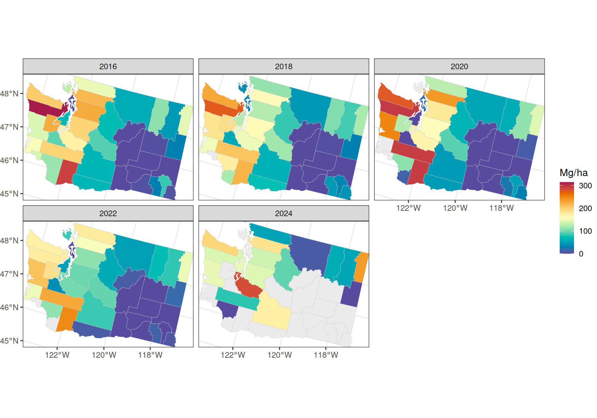
The map below shows model-ready direct estimates for selected years. These are county-year sample means of agb_live_mg_ha with model-ready variance handling for the area-response articles.
7 Plot-Value Snapshot
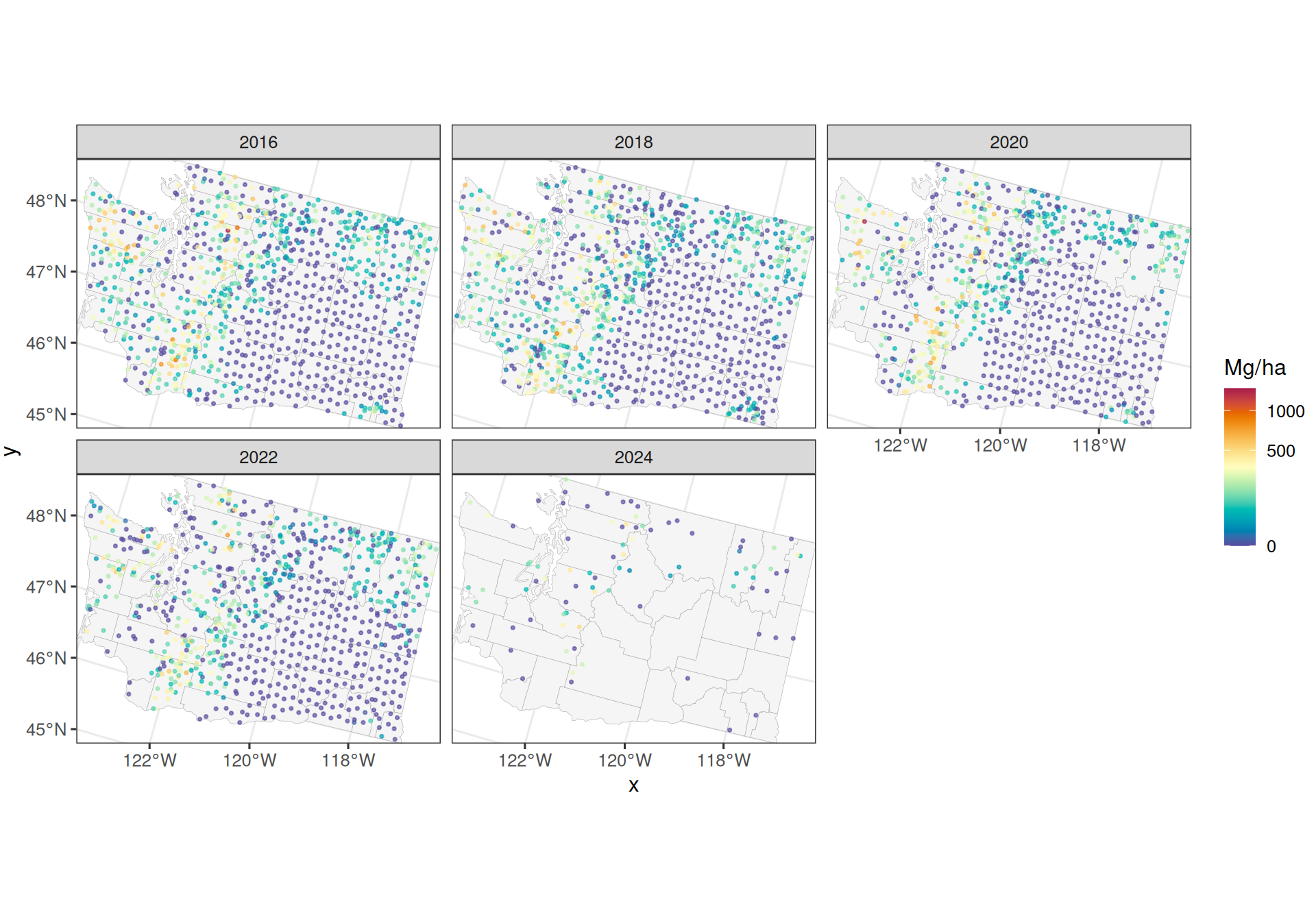
The map below shows the plot-level response used by the unit-response articles. The direct estimates above are county-year sample means of the same variable.
8 County Mean TCC
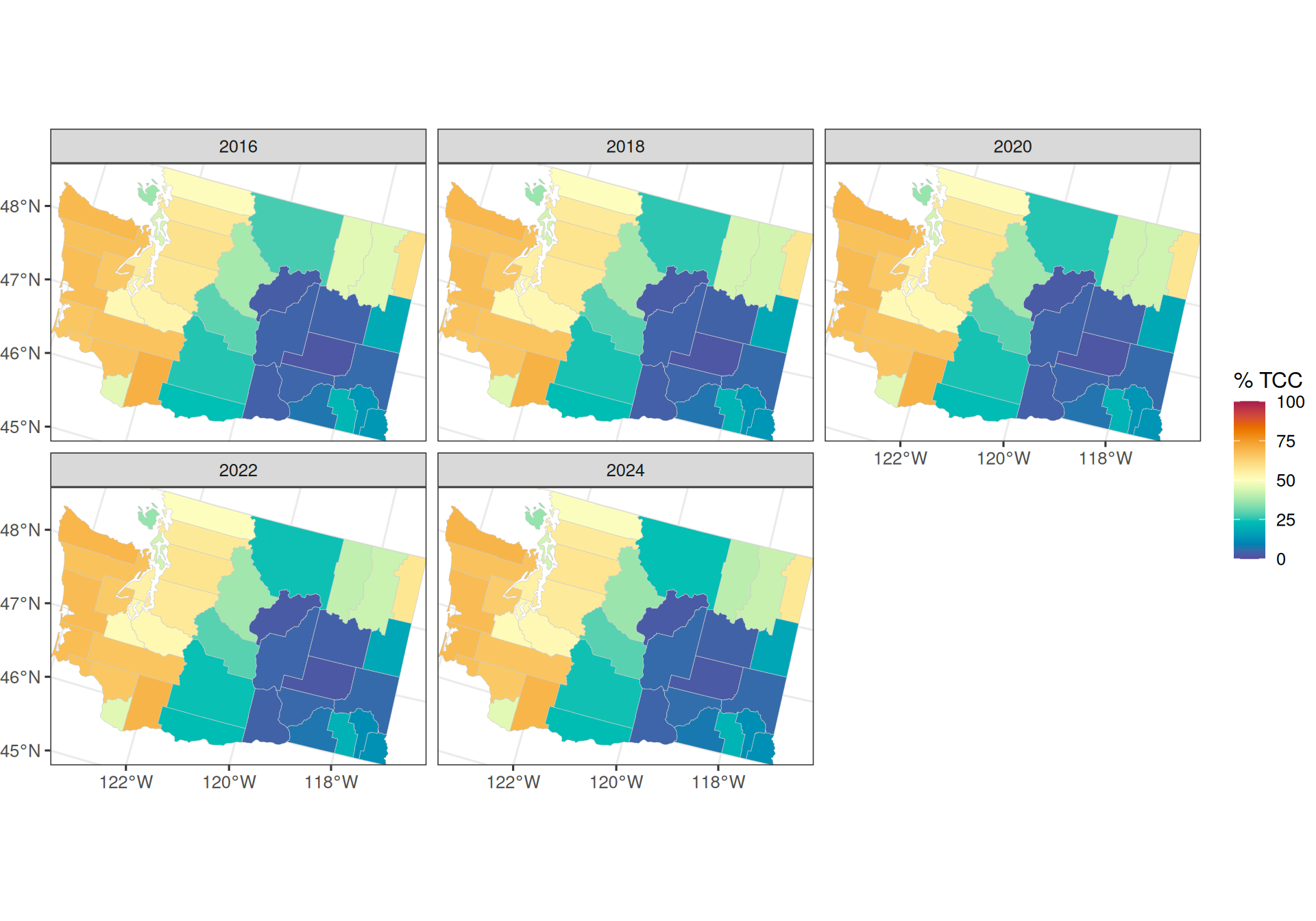
County-year mean TCC is the area-level covariate used in the direct-estimate models. It summarizes the annual TCC raster within each county.
9 Prediction Grid TCC
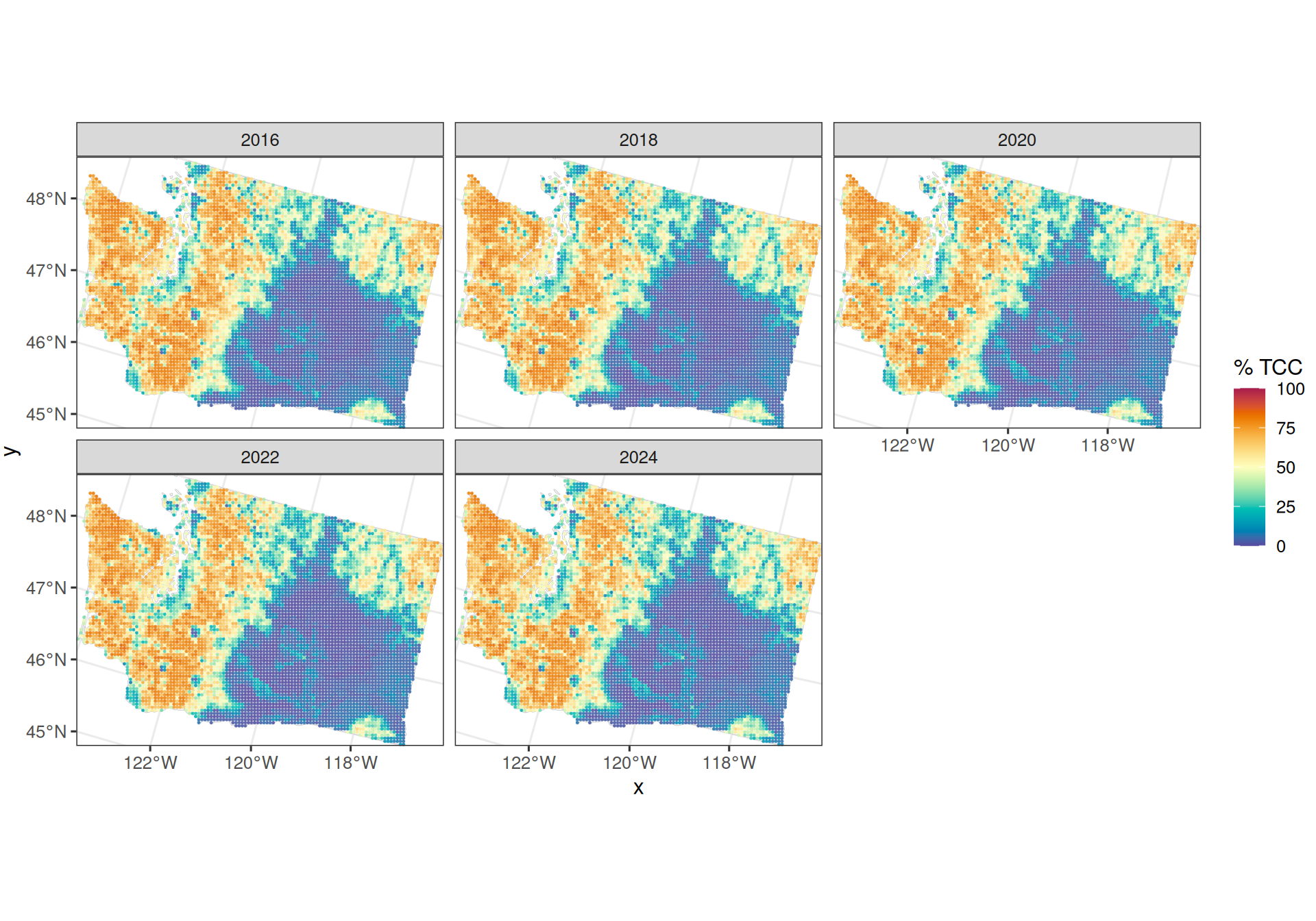
Unit-level prediction uses grid rows that inherit county and FIA-unit labels. The article data bundle includes 5 km and 10 km grid files. The full grids are systematic in the projected coordinate system. The 5 km grid is the default grid for model articles, and the 10 km grid is useful for faster checks.
10 Reading the Model Sequence
The articles that follow build the models as a ladder. Each step changes one part of the analysis, such as the smoothing structure, the TCC covariate, the observation-variance model, or the unit-level response formulation. Reading across the series helps make those choices visible.
Model results will be reported on a common county-year scale so the articles can be compared directly. The main summaries are:
- posterior mean, median, and 95% credible interval for the county-year mean of
agb_live_mg_ha; - direct-estimate information where it is available;
- posterior uncertainty summaries on the same Mg/ha scale;
- the response and aggregation target used by the model: area-level direct estimates, single-stage unit responses, or positive-biomass two-stage unit responses.
The sequence is meant to support a few practical questions:
- How much smoothing does the model add relative to the direct estimates?
- How much do TCC covariates change county-year predictions?
- Where do spatial and space-time effects matter most?
- Does FIA-unit heteroskedasticity change uncertainty in a visible way?
- How different are single-stage Gaussian estimates from positive-biomass two-stage estimates for the same series target?
The goal is not to choose one universal best model. The series is meant to show what each model assumes, where it borrows strength, what auxiliary information it uses, and how those choices affect county-level forest inventory inference.
The Colville capstone returns to part of the question deferred in this overview: what changes when the target follows FIA forestland definitions rather than the simplified working target used in the model tour? That article looks at forestland support, a user-defined spatial extent, and a two-stage unit-response formulation for biomass on forested land rather than a simplified county-year mean.