Code
system.file("doc", "cosTapered.pdf", package = "cosTapered")
Model notation, MCMC, prediction targets, and practical support guidance
Source:vignettes/cosTapered-model.qmd
This vignette gives the statistical and computational details behind cosTapered. It is the technical companion to the introductory vignette. The introductory vignette shows the user workflow; this vignette explains the model parameterization, support averaging, nugget scaling, collapsed sampler, recovery distributions, prediction targets, and computational tradeoffs.
The Gaussian implementation described below supports a tapered exponential Gaussian process, proper normal regression priors, inverse-gamma variance priors, a bounded uniform prior for the exponential decay parameter, simple S3 objects, and latent or observed prediction targets.
The separate cosTapered-binomial and cosTapered-negative-binomial vignettes illustrate the experimental Polya-Gamma response paths. The negative-binomial path supports fixed-size count responses with user-supplied offsets such as log exposure.
For readers who want the model notation and posterior calculations in one place, the repository includes a PDF model and software details document. After installing with build_vignettes = TRUE, locate it with:
system.file("doc", "cosTapered.pdf", package = "cosTapered")Let A_i, i=1,\ldots,n_A, denote raster cells on the fine support. Let s_i be the centroid of A_i. Let B_l, l=1,\ldots,n_B, denote observed supports, and let U_k, k=1,\ldots,n_U, denote areal prediction supports.
The fine-support covariate vector for cell A_i is \mathbf{x}(A_i)\in\mathbb{R}^p, and the fine-support covariate matrix is
X = \begin{bmatrix} \mathbf{x}(A_1)^\top\\ \vdots\\ \mathbf{x}(A_{n_A})^\top \end{bmatrix}.
The package uses the columns supplied in X_rast. If an intercept is desired, the user supplies an intercept raster layer.
Observed-support area weights are
h_{li} = \frac{|B_l\cap A_i|}{|B_l|},
where |\cdot| denotes area. The observed-support aggregation matrix is H_{BA} with entries h_{li}. Prediction-support area weights are
g_{ki} = \frac{|U_k\cap A_i|}{|U_k|},
and define the conceptual aggregation matrix H_{UA}. In the implementation, cos_prepare() stores H_{BA} as a sparse matrix, while cos_make_areal_blocks() stores prediction weights block by block.
The fine-support response is decomposed into a latent mean and independent finite-support noise:
y(A_i) = \eta(A_i) + \epsilon(A_i), \qquad \eta(A_i) = \mathbf{x}(A_i)^\top\beta+\omega(A_i).
In vector form,
\mathbf{y}_A = \boldsymbol{\eta}_A+\boldsymbol{\epsilon}_A, \qquad \boldsymbol{\eta}_A = X\beta+\boldsymbol{\omega}_A,
with
\boldsymbol{\epsilon}_A\mid\tau^2 \sim N(0,\tau^2 I_{n_A}).
The noise term is a finite raster-cell noise term. It is not a continuous point-level white-noise process. This matters because observed-support nugget variance is obtained by averaging finite-cell noise terms through the support weights.
The residual spatial process is Gaussian:
\boldsymbol{\omega}_A\mid\sigma^2,\phi,\gamma \sim N\{0,\sigma^2 C_A^{tap}(\phi,\gamma)\},
where
[C_A^{tap}(\phi,\gamma)]_{ij} = \exp\{-\phi d(s_i,s_j)\}T_\gamma\{d(s_i,s_j)\}.
Here d(s_i,s_j) is Euclidean distance in the projected coordinate system, \phi>0 is the exponential decay parameter, and \gamma>0 is the taper distance. The taper distance is a hard covariance cutoff: if d(s_i,s_j)\geq\gamma, the tapered covariance contribution is zero.
The package currently supports two compact tapers. For taper_code = 1L, the Wendland taper is
T_\gamma(d) = \begin{cases} (1-r)^4(1+4r), & 0\leq r < 1,\\ 0, & r\geq 1, \end{cases} \qquad r=d/\gamma.
For taper_code = 2L, the spherical taper is
T_\gamma(d) = \begin{cases} 1 - 1.5r + 0.5r^3, & 0\leq r < 1,\\ 0, & r\geq 1. \end{cases}
The exponential effective range reported by the package is the distance at which the exponential component alone drops to 0.05:
\exp(-\phi r_{0.05})=0.05, \qquad r_{0.05}=-\log(0.05)/\phi\approx 3/\phi.
The reported effective range is not the taper distance. The taper distance \gamma controls compact support of the covariance and must be chosen by the user.
Observed responses are modeled as support averages of the fine-support response:
y(B_l) \approx \sum_{i=1}^{n_A} h_{li} y(A_i).
Stacking observed responses gives
\mathbf{y}_B = H_{BA}X\beta + H_{BA}\boldsymbol{\omega}_A + H_{BA}\boldsymbol{\epsilon}_A.
Define
X_B = H_{BA}X, \qquad \boldsymbol{\omega}_B = H_{BA}\boldsymbol{\omega}_A, \qquad D_h = H_{BA}H_{BA}^\top.
Then
\mathbf{y}_B\mid\beta,\boldsymbol{\omega}_B,\tau^2 \sim N(X_B\beta+\boldsymbol{\omega}_B,\tau^2D_h).
The observed-support spatial effects have prior
\boldsymbol{\omega}_B\mid\sigma^2,\phi,\gamma \sim N\{0,\sigma^2C_B^{tap}(\phi,\gamma)\},
where
C_B^{tap}(\phi,\gamma) = H_{BA}C_A^{tap}(\phi,\gamma)H_{BA}^\top.
Only fine-cell pairs with d(s_i,s_j)<\gamma contribute. The package uses this to precompute the contributing support-pair pattern for fixed observed supports, raster cells, taper type, and taper distance. During MCMC, the code rebuilds C_B^{tap}(\phi,\gamma) by applying \exp(-\phi d) to precomputed distances and taper weights.
The model is written in terms of the fine-support noise variance \tau^2. However, observed data see this noise through \tau^2D_h. The package therefore places the prior and MCMC proposal on the average observed-support nugget variance
\tau_B^2 = \tau^2\bar d_h, \qquad \bar d_h = \frac{1}{n_B}\sum_{l=1}^{n_B}D_h(l,l).
Thus
\tau^2=\tau_B^2/\bar d_h.
This is a reparameterization of the same model. It does not imply that every observed support has nugget variance \tau_B^2. For observed support B_l,
\mathrm{var}\{(H_{BA}\boldsymbol{\epsilon}_A)_l\} = \tau^2D_h(l,l) = \frac{\tau_B^2}{\bar d_h}D_h(l,l).
When observed supports do not overlap in raster cells, D_h is diagonal. If supports overlap, D_h can have nonzero off-diagonal entries. The package uses the general matrix expression.
The regression prior is proper normal:
\beta\sim N(\mu_\beta,V_\beta).
The variance priors use inverse-gamma distributions in shape-scale form:
\tau_B^2 \sim \mathrm{IG}(a_\tau,b_\tau), \qquad \sigma^2 \sim \mathrm{IG}(a_\sigma,b_\sigma),
where
p(x) = \frac{b^a}{\Gamma(a)} x^{-(a+1)} \exp(-b/x), \qquad x>0.
For spatial fits,
\phi\sim \mathrm{Uniform}(\phi_L,\phi_U), \qquad 0<\phi_L<\phi_U<\infty.
Bounds can be chosen through approximate exponential effective ranges:
\phi_L=3/r_{\max}, \qquad \phi_U=3/r_{\min}.
cos_fit() samples covariance parameters from a collapsed posterior in which \beta and, for spatial fits, \boldsymbol{\omega}_B have been integrated out. For spatial fits define
\theta_B=(\tau_B^2,\sigma^2,\phi).
For each proposed \tau_B^2, the package converts to \tau^2=\tau_B^2/\bar d_h before constructing the covariance.
After integrating over \beta and \boldsymbol{\omega}_B,
\mathbf{y}_B\mid\theta_B \sim N(\mu_Y,V_Y),
where
\mu_Y = X_B\mu_\beta,
and
V_Y = X_BV_\beta X_B^\top + \sigma^2C_B^{tap}(\phi,\gamma) + \tau^2D_h.
Thus the collapsed posterior density is proportional to
p(\theta_B\mid\mathbf{y}_B) \propto N(\mathbf{y}_B\mid\mu_Y,V_Y) p(\tau_B^2)p(\sigma^2)p(\phi).
For nonspatial fits, \boldsymbol{\omega}_B is omitted and
V_Y = X_BV_\beta X_B^\top+\tau^2D_h.
The package evaluates the Gaussian log density using a Cholesky factorization of the n_B\times n_B matrix V_Y. This is the main fitting cost for moderate or large n_B.
The sampler works on an unconstrained scale. For spatial fits,
z_\tau = \log\tau_B^2, \qquad z_\sigma = \log\sigma^2, \qquad z_\phi = \log\left(\frac{\phi-\phi_L}{\phi_U-\phi}\right).
The inverse transformation is
\tau_B^2=\exp(z_\tau), \qquad \sigma^2=\exp(z_\sigma), \qquad \phi=\phi_U-\frac{\phi_U-\phi_L}{1+\exp(z_\phi)}.
For the range parameter,
\frac{d\phi}{dz_\phi} = \frac{(\phi-\phi_L)(\phi_U-\phi)}{\phi_U-\phi_L}.
Thus, after dropping additive constants that do not affect Metropolis acceptance probabilities, the transformed log target includes
\log(\phi-\phi_L) + \log(\phi_U-\phi)
for the bounded transformation of \phi. The full transformed target also includes the log-Jacobian terms \log\tau_B^2 and \log\sigma^2 for the log variance transformations. For nonspatial fits, the sampler uses only z_\tau=\log\tau_B^2.
The internal sampler uses a random-walk block proposal and adapts a scalar multiplier and covariance shape by batch. The package stores both natural-scale samples and unconstrained-scale samples.
After fitting, cos_recover_B() retains a subset of covariance parameter samples according to burn_in, thin, and optional n_samples. For each retained draw, it samples \beta and \boldsymbol{\omega}_B from their Gaussian full conditional.
For spatial fits, define
\alpha = \begin{bmatrix} \beta\\ \boldsymbol{\omega}_B \end{bmatrix}, \qquad Z=[X_B,I_{n_B}].
The likelihood is
\mathbf{y}_B\mid\alpha,\tau^2 \sim N(Z\alpha,\tau^2D_h).
The prior is block Gaussian:
\alpha \sim N\left[ \begin{bmatrix} \mu_\beta\\ 0 \end{bmatrix}, \begin{bmatrix} V_\beta & 0\\ 0 & \sigma^2C_B^{tap}(\phi,\gamma) \end{bmatrix} \right].
Therefore
\alpha\mid\mathbf{y}_B,\theta_B \sim N(Q_\alpha^{-1}b_\alpha,Q_\alpha^{-1}),
where
Q_\alpha = \frac{1}{\tau^2}Z^\top D_h^{-1}Z + \begin{bmatrix} V_\beta^{-1} & 0\\ 0 & \sigma^{-2}\{C_B^{tap}(\phi,\gamma)\}^{-1} \end{bmatrix}.
The corresponding information vector is
b_\alpha = \frac{1}{\tau^2} Z^\top D_h^{-1}\mathbf{y}_B + \begin{bmatrix} V_\beta^{-1}\mu_\beta\\ 0 \end{bmatrix}.
Here burn_in is the first retained iteration within each chain, and n_samples caps the total number of retained draws across chains.
The implementation samples from this conditional distribution using a Cholesky factorization of Q_\alpha. It stores draws of \beta, \boldsymbol{\omega}_B, and the observed-support latent mean
\eta_B=X_B\beta+\boldsymbol{\omega}_B.
For nonspatial fits, \boldsymbol{\omega}_B=0 and only \beta is recovered.
Fine-support prediction is implemented by cos_predict_fine(). Its default locations are the complete raster cells intersecting the observed supports. Supply both pred_coords and X_pred to predict elsewhere, including over the full raster domain. For prediction locations P, let X_P be the prediction covariate matrix and let \boldsymbol{\omega}_P be the corresponding spatial residual vector. For a retained posterior draw,
\boldsymbol{\omega}_P \mid \boldsymbol{\omega}_B,\sigma^2,\phi,\gamma \sim N\{C_{PB}C_B^{-1}\boldsymbol{\omega}_B,\, \sigma^2(C_{PP}-C_{PB}C_B^{-1}C_{BP})\}.
The latent fine-support target is
\eta_P = X_P\beta+\boldsymbol{\omega}_P.
By default, spatial_uncertainty = "conditional_mean": the package uses the conditional mean of \boldsymbol{\omega}_P, so uncertainty summaries omit conditional spatial prediction uncertainty. With spatial_uncertainty = "marginal", it draws independent marginal conditional values for each fine prediction location. With spatial_uncertainty = "joint", it draws from the full joint conditional distribution across the fine prediction locations, which can be expensive for large prediction sets.
For target = "observed", the package adds independent nugget draws:
y_P = \eta_P+\epsilon_P, \qquad \epsilon_P\sim N(0,\tau^2I).
For areal prediction unit U_k, the latent target is the support average
\eta(U_k) = \sum_i g_{ki}\eta(A_i).
For target = "observed", the observed support prediction is
y(U_k)=\eta(U_k)+\epsilon(U_k),
where
\epsilon(U_k)\sim N\left(0,\tau^2\sum_i g_{ki}^2\right).
The package reports areal means, not totals. Users should multiply by their chosen area units outside the package if totals are needed.
For areal prediction, spatial_uncertainty = "conditional_mean" uses conditional means of the unobserved areal spatial effects and therefore omits conditional spatial prediction uncertainty. spatial_uncertainty = "marginal" adds marginal conditional uncertainty for each areal unit, but those samples are not joint samples across units. They should not be used for totals, contrasts, rankings, or other summaries that require cross-unit posterior covariance.
Prediction has three separate choices: support, response target, and spatial uncertainty. Keeping those choices separate makes the estimand explicit. Choose the combination that matches the inferential target first; runtime is secondary. For Gaussian fits, target = "latent" estimates the underlying support mean, excluding nugget variation. This is usually the target for stand, polygon, inventory, and mapped-condition summaries. target = "observed" adds the Gaussian nugget contribution on the requested support, so it targets the observed response on that support rather than the underlying support mean. For statistically coherent estimates of individual stands, polygons, or cells with posterior SDs and intervals, use spatial_uncertainty = "marginal". That option gives valid marginal summaries for each unit considered separately. It does not give joint samples across units, so it is not appropriate for totals, rankings, contrasts, or allocation rules that need cross-unit posterior covariance.
If the target is a collection of stands or polygons as one aggregate estimand, first dissolve those boundaries to the union support and predict that union. Do not create uncertainty for the collection by adding independently drawn marginal predictions from separate stands.
The figure below summarizes the Gaussian and binomial spatial-uncertainty paths. Negative-binomial prediction follows the same Polya-Gamma conditional_mean or marginal spatial-uncertainty choices as binomial, with mean-count summaries for target = "latent" and count draws for target = "observed".
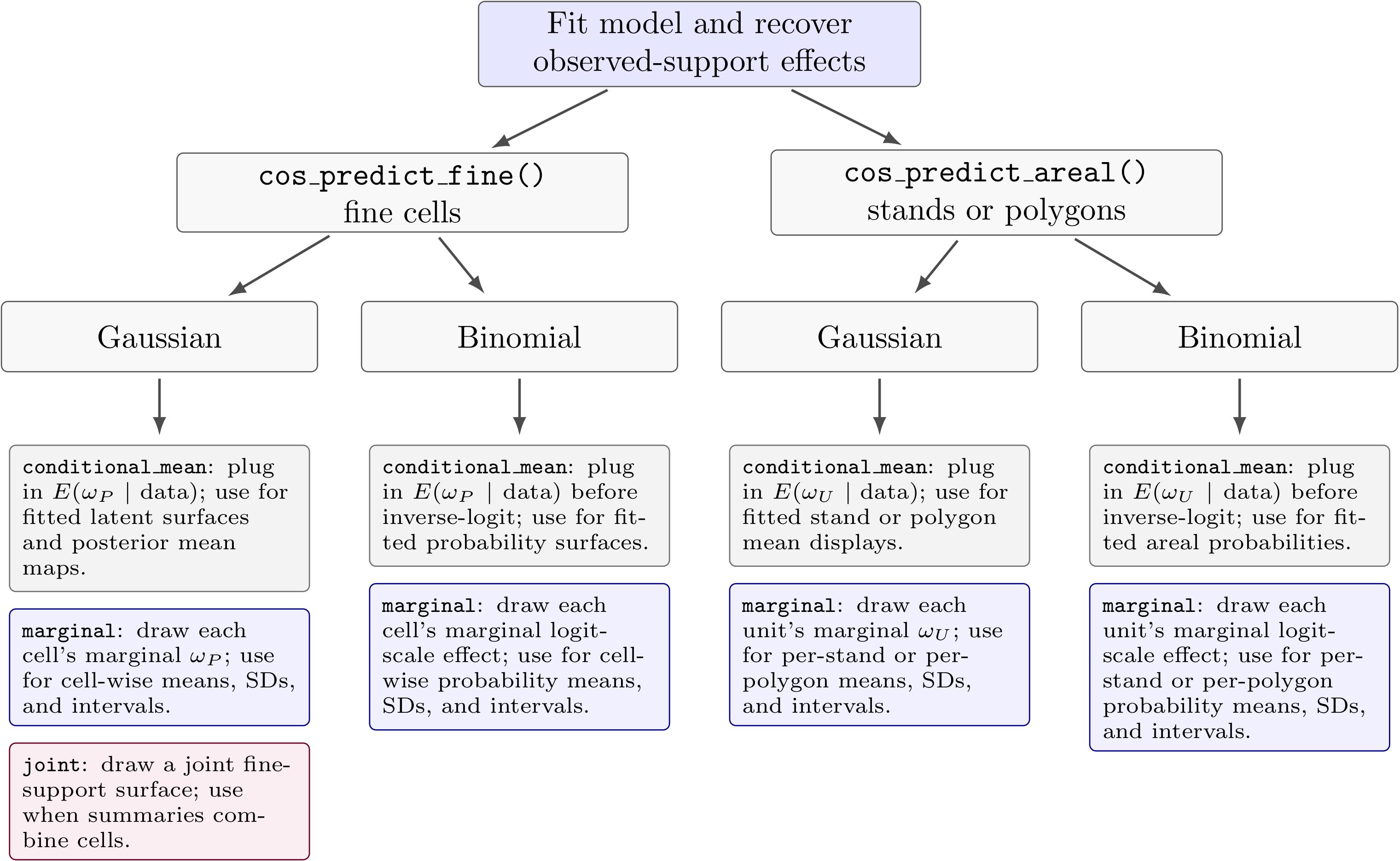
The choices mean:
target = "latent" summarizes the underlying support mean on the model scale.target = "observed" adds the Gaussian nugget contribution on the requested support: fine-cell nugget variation for fine predictions and support-averaged nugget variation for areal predictions. For negative-binomial fits, target = "observed" simulates count draws around the latent mean.spatial_uncertainty = "conditional_mean" plugs in the conditional mean of unobserved spatial effects. It is a fitted-surface or plug-in summary, not a full prediction-uncertainty summary.spatial_uncertainty = "marginal" draws independent marginal conditional spatial effects for each prediction cell or unit. It is the right choice for valid per-cell, per-stand, or per-polygon means, SDs, and intervals when units are interpreted separately.spatial_uncertainty = "joint" draws a joint Gaussian fine-support surface and is available for Gaussian fine prediction only. Use it when the summary combines fine cells and therefore depends on cross-cell covariance.With keep_samples = FALSE, prediction returns posterior means and SDs. Set keep_samples = TRUE to also retain samples and compute the 2.5%, 50%, and 97.5% posterior quantiles.
Support weights define the estimand. If an observed or prediction support overlaps raster cells with incomplete covariates, simply dropping those cells changes the support average. For this reason, cos_prepare() and cos_make_areal_blocks() default to missing = "error" when incomplete covariates would leave support-weight rows below one. Users can choose missing = "drop" to keep covered-cell weights without rescaling, or missing = "renormalize" to average over covered cells only. Those choices should be made deliberately because they change the target support.
cos_cv_observed() provides the Gaussian observed-support K-fold workflow. For each fold it refits the model to training polygons, treats held-out polygons as prediction units, predicts their latent areal means, optionally adds observed-support nugget draws, and scores posterior predictive samples.
The function can score:
target = "latent" against known latent truth in simulation studies;target = "observed" against held-out observed responses;target = c("latent", "observed") and latent_col is supplied.This target distinction is important. Latent prediction checks whether the model recovers the support-averaged spatial mean. Observed prediction checks the response on that support with nugget variation included.
The main fitting cost is repeated Cholesky factorization of the observed-level matrix V_Y. The main spatial-preparation cost is computing the support-pair contributions within taper distance \gamma. Larger \gamma values can improve fidelity to long-range residual dependence, but they increase the number of contributing fine-cell pairs and therefore memory and time.
Useful practical checks are:
gamma large enough to cover residual spatial dependence that matters for prediction;phi bounds using plausible effective ranges;phi is not stuck against a bound;For applied guidance on when spatial COS should improve prediction, see the spatial-guidance vignette.