| Model | Fold fits | Maximum R-hat | Minimum bulk ESS | Minimum tail ESS |
|---|---|---|---|---|
| nonspatial | 900 | 1.0049 | 2318 | 1867 |
| spatial | 900 | 1.0099 | 517 | 402 |
When Should the Spatial COS Model Improve Prediction?
Range, target support, scoring rules, and practical model choice
Source:vignettes/cosTapered-spatial-guidance.qmd
1 What this article can tell you
Spatial COS is useful when residual spatial dependence lets observed supports inform prediction supports after accounting for covariates. Whether that happens depends on the sampling layout, support sizes, covariance, and prediction target. An effective range in meters is not a universal model-selection rule.
This article combines practical guidance with a reproducible Gaussian simulation example. It compares spatial and nonspatial COS on identical held-out plots, includes a case with no spatial effect, and checks sensitivity to prior scales. The simulation is deliberately limited to one landscape and one plot design; it does not establish performance for binomial or negative-binomial models, other landscapes, or spatial extrapolation.
The main steps for an applied analysis are:
- Define whether the target is a latent support mean or an observed response.
- Fit a nonspatial COS baseline with the same covariates and support weights.
- Evaluate the spatial model on validation splits that resemble the intended prediction task.
- Compare prediction error and predictive distributions, including interval width and coverage together.
- Check posterior sampling and whether the conclusion depends on the priors.
2 Match the prediction target to the question
For an observed support B_l, the Gaussian latent mean is
\eta(B_l) = \sum_i h_{li}\{x(A_i)^\top\beta + \omega(A_i)\}.
The measured response is
\begin{aligned} y(B_l) &= \eta(B_l) + \epsilon(B_l),\\ \operatorname{Var}\{\epsilon(B_l)\} &= \tau^2 \sum_i h_{li}^2. \end{aligned}
The weights h_{li} connect the fine raster cells to the observed support. The nugget formula assumes independent fine-cell nugget terms. The same expressions apply to a new areal unit U_k using its weights g_{ki}.
Use target = "latent" for the underlying support mean. Use target = "observed" for a response that includes nugget variation. The latter needs wider predictive intervals because the nugget is not known.
In this simulation both targets are known, so they can be scored separately. In ordinary observed-data cross-validation, score observed predictions against held-out responses. A held-out noisy response is not ground truth for a latent mean. The package requires a latent_col containing a known latent target when cos_cv_observed() scores target = "latent".
For uncertainty at an individual prediction unit, request spatial_uncertainty = "marginal"; the prediction functions’ default "conditional_mean" omits conditional variation in the unobserved spatial effect. The CV function requests marginal uncertainty internally. Retaining prediction draws and quantiles also requires keep_samples = TRUE. Marginal areal draws do not supply the joint uncertainty needed for stand contrasts, rankings, or totals across units.
3 A controlled simulation comparison
The study uses fixed priors independent of all responses, a fixed taper distance, multiple chains, and recorded convergence diagnostics. All numerical summaries and figures below are generated from archived results.
The canopy raster is averaged from 3 m to 12 m cells to make a repeated study practical. All simulation, fitting, and prediction calculations use this coarser fine-support grid. These results therefore concern this grid, not the original 3 m analysis. Circular plots have a target radius of 16 m and are clipped at the forest boundary. The layout and CV folds stay fixed.
| Setting | Value |
|---|---|
| Observed plots | 49 |
| Replicates per generating case | 10 independent simulated datasets |
| Validation | 5 random folds, identical for both models |
| Spatial cases | Nominal exponential ranges 50, 150, 350, 750, and 1000 m |
| Nonspatial truth case | \sigma^2=0 |
| Spatial truth cases | \sigma^2=750 |
| Nugget scale | \tau_B^2=250, the average observed-support nugget variance |
| Regression coefficients | \beta=(-10,\ 15.87132)^\top |
| Taper | Wendland, fixed \gamma=1500 m in every case |
| Prior sensitivity | Inverse-gamma scales 250, 500, and 1000 |
Here 3/\phi is the nominal exponential range, where the exponential component alone is about 0.05. Multiplying by the taper lowers correlation further. Holding \gamma fixed separates changes in exponential range from changes in the taper cutoff. The fitted spatial models estimate \phi; the true range is never supplied to their fitting priors or starting values. Although fine-support \sigma^2 is fixed in the spatial cases, support averaging attenuates short-range variation more strongly. Thus the areal signal-to-noise ratio varies with range even though \sigma^2 is fixed.
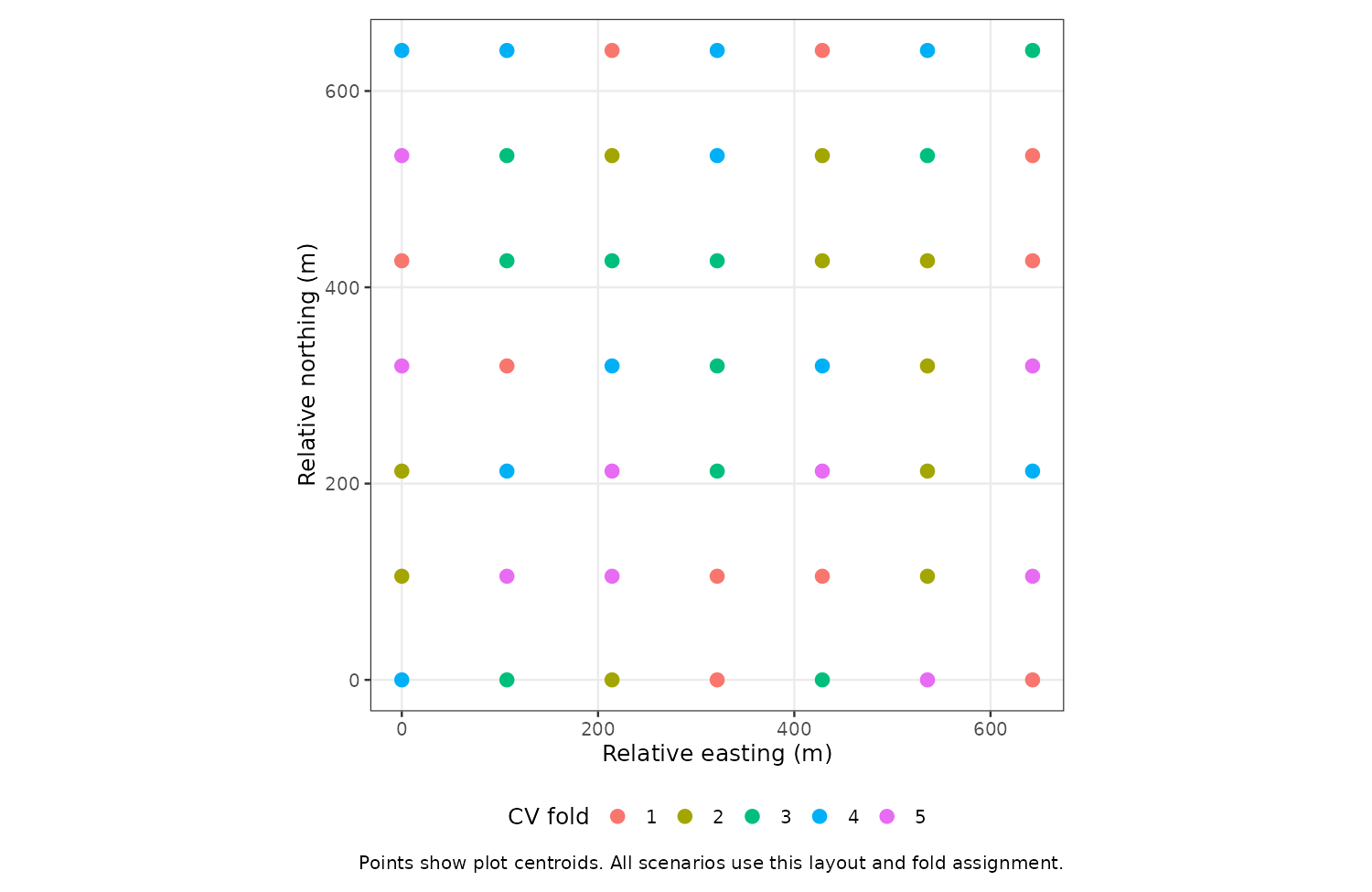
For this design, the median distance from a held-out plot centroid to the nearest training plot centroid is 107 m (range 106–107 m). The folds assess predictions among interspersed observed plots. Predicting into distant unsampled regions calls for a different validation design; these results do not measure that task.
3.1 Priors and fitting
Both models use the same regression prior, \beta\sim N\{(0,0)^\top,\operatorname{diag}(100^2,10^2)\}, and the same observed-support nugget prior \tau_B^2\sim\operatorname{IG}(2,b). The spatial model additionally uses \sigma^2\sim\operatorname{IG}(2,b) and a uniform prior on \phi\in[3/1500,3/10].
The primary comparison uses b=500. Repeating it with b=250 and b=1000 checks sensitivity on the same data and folds. These are specified study priors, not estimates from the simulated responses or their generating parameters. Shared-parameter priors are identical across models, but the extra spatial variance component means their full prior predictive distributions are not identical. Choose priors appropriate to the response and distance units in your own analysis; these particular scales are choices for the simulation example.
cos_cv_observed() reuses the supplied fit’s priors in every fold. That is appropriate here because these priors do not depend on responses. If prior scales are estimated from response data, an explicit fold loop must estimate them from the training observations only. Calculating var(y) on the complete dataset before cross-validation lets held-out responses influence the fitted models.
Every fold is refitted with four chains from dispersed, prespecified starting values. The first half of each chain is discarded. The script checks rank-normalized split R-hat below 1.01 and bulk and tail effective sample sizes of at least 400 for each sampled covariance parameter and log posterior. These checks use the unthinned retained chains. Failed checks trigger longer runs; unresolved failures stop publication of the figures. Diagnostics use the posterior package.
Final runs used 10,000 to 40,000 iterations per chain. Approximately 2000 posterior predictive draws were used per held-out plot. Passing these diagnostics is a useful check on computation, not proof of model adequacy or a guarantee that all Monte Carlo error is negligible.
4 Prediction accuracy and uncertainty
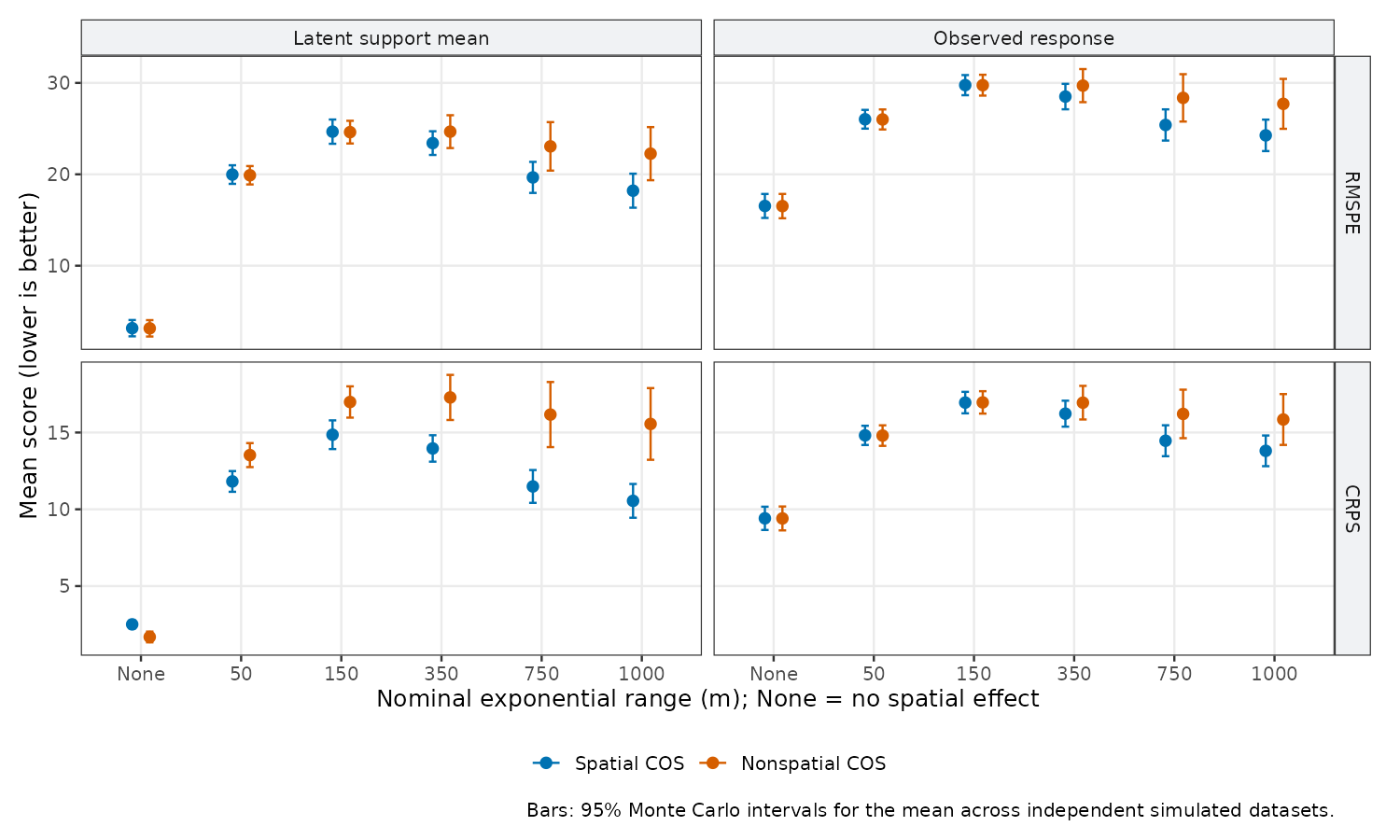
RMSPE measures point-prediction error; lower is better. CRPS scores the predictive distribution; lower is better. The study first scores all held-out plots within a simulated dataset, then averages those dataset-level scores. Its Monte Carlo uncertainty treats each simulated dataset as one replicate; it does not treat folds or plots as independent simulation replicates. Error bars use the mean plus or minus a Student-t multiplier times the simulation SE, with 9 degrees of freedom. They are approximate 95% intervals for mean performance under this fixed design.
For each replicate, percentage improvement is
100\,\frac{\mathrm{score}_{\mathrm{nonspatial}}- \mathrm{score}_{\mathrm{spatial}}} {\mathrm{score}_{\mathrm{nonspatial}}}.
Positive values favor spatial COS. The table reports the mean of these paired percentages and its simulation standard error (SE). It is not a percentage computed from the two grand mean scores.
| Case | Target | RMSPE gain (%) | CRPS gain (%) | RMSPE win rate |
|---|---|---|---|---|
| No spatial effect | latent | -0.6 (SE 0.9) | -55.4 (SE 8.9) | 40% |
| No spatial effect | observed | -0.1 (SE 0.1) | -0.1 (SE 0.2) | 40% |
| 50 m | latent | -0.4 (SE 0.2) | 12.7 (SE 0.4) | 20% |
| 50 m | observed | -0.1 (SE 0.2) | -0.1 (SE 0.3) | 50% |
| 150 m | latent | -0.2 (SE 0.5) | 12.6 (SE 0.5) | 50% |
| 150 m | observed | -0.0 (SE 0.4) | 0.0 (SE 0.4) | 60% |
| 350 m | latent | 4.7 (SE 1.9) | 18.7 (SE 2.2) | 80% |
| 350 m | observed | 3.7 (SE 1.9) | 3.9 (SE 2.0) | 80% |
| 750 m | latent | 12.9 (SE 4.9) | 26.7 (SE 5.0) | 90% |
| 750 m | observed | 9.2 (SE 4.2) | 9.4 (SE 4.4) | 80% |
| 1000 m | latent | 15.9 (SE 5.5) | 29.4 (SE 5.4) | 100% |
| 1000 m | observed | 10.9 (SE 4.6) | 11.3 (SE 4.6) | 80% |
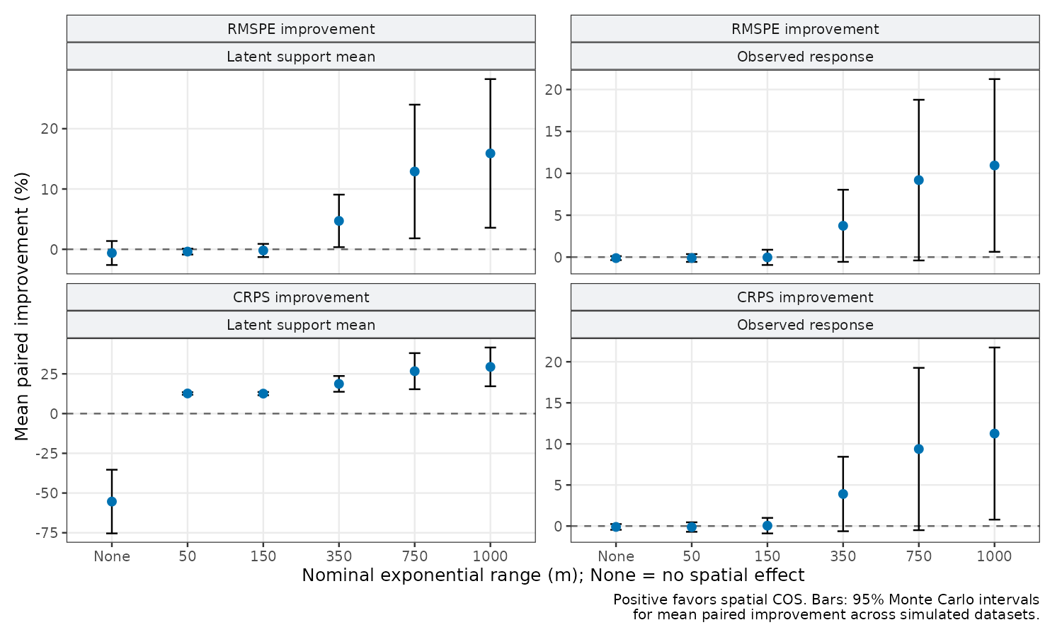
In this run, RMSPE differences at 50 and 150 m are close to zero. Average gains increase at the longer ranges. At 1000 m the mean paired RMSPE improvement is 15.9% for latent means and 10.9% for observed responses, with simulation SEs of 5.5 and 4.6 percentage points. The uncertainty around these averages is substantial; the point estimates are not guaranteed gains for a new dataset.
Latent CRPS favors spatial COS in the spatial truth cases, including the short-range cases where point predictions barely change. The spatial model represents uncertainty about an unobserved spatial effect that the nonspatial latent mean omits. For observed responses, CRPS is essentially tied at short ranges and improves on average at longer ranges.
The nonspatial truth case shows the other side of the comparison. Under these priors, point prediction is similar, but the spatial model’s extra latent uncertainty worsens latent CRPS. Read the absolute scores alongside percentages: a modest absolute difference can be a large percentage when the baseline score is small.
4.1 Coverage must be read with interval width
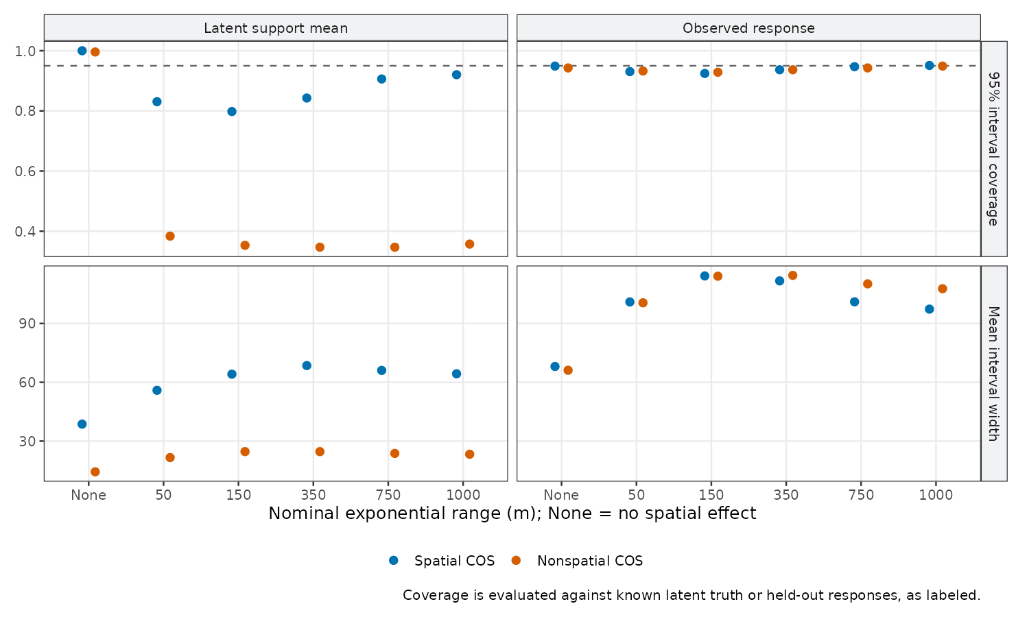
The spatial model’s latent intervals still under-cover in this study: mean coverage across the spatial truth cases ranges from 79.8% to 92%, below the nominal 95%. These are repeated-simulation coverage rates at fixed generating parameters; a 95% posterior interval does not automatically attain 95% coverage in that experiment. Better CRPS and satisfactory chain diagnostics do not establish calibrated intervals. At ranges shorter than the plot spacing, the data contain little correlation information to separate spatial variance from nugget variance; the prior choices can matter substantially.
Observed-response coverage is closer to nominal for both models, ranging from 92.4% to 95.1% across cases in the primary comparison. Spatial observed-response intervals become narrower at the longer ranges, while their short-range widths are similar to the nonspatial intervals.
For latent truth, nonspatial COS predicts X_B\beta, whereas spatial truth also contains \omega_B. Nonspatial latent intervals need not cover this omitted component. Poor latent coverage under spatial truth should not be interpreted as a general failure of nonspatial regression intervals to cover their own model’s mean.
For observed responses, the nonspatial model can absorb unexplained variation into its nugget. Whether this gives suitable coverage and useful interval width is an empirical question. A nominal 95% interval with coverage near 1 is conservative in this study; high coverage alone is not evidence of better uncertainty quantification. Compare the width, CRPS, and prediction errors too.
4.2 Does the conclusion depend on the prior?
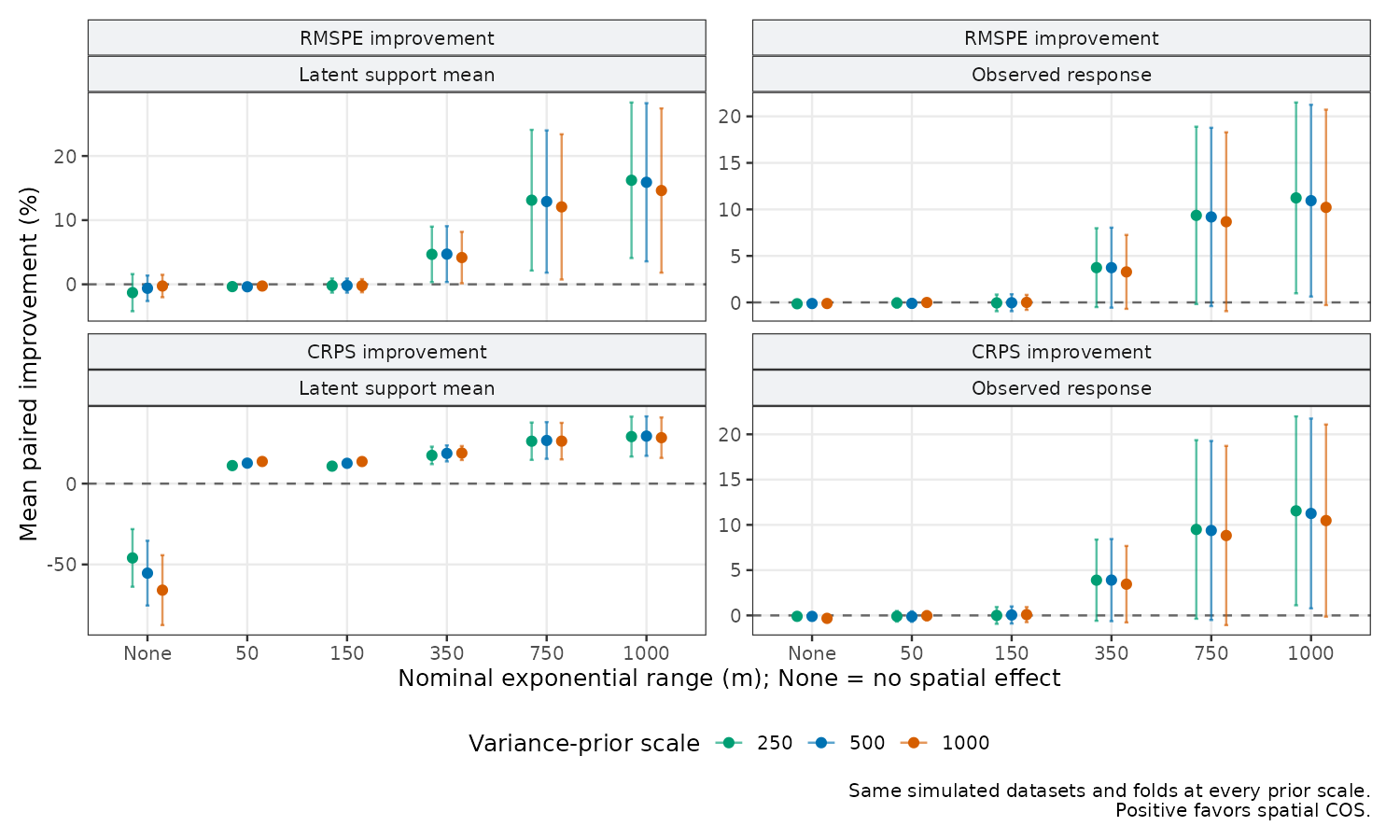
Changing the variance-prior scale does not reverse the near-ties in point prediction at 50 and 150 m or the mean advantage at 1000 m. At 1000 m, mean paired observed-response RMSPE improvements range from 10.2–11.2% across the three scales. The simulation uncertainty around these estimates remains substantial.
The latent predictive distribution is more sensitive. At 50 m, the spatial model’s latent interval coverage ranges from 80.4–85.3% across the priors, still below 95%. In the no-spatial-effect case, its latent CRPS is 46.0–65.9% worse than the nonspatial baseline. Increasing the variance-prior scale widens latent intervals in these two cases: that helps coverage under spatial truth but adds unnecessary uncertainty under nonspatial truth. A prior choice that leaves point predictions nearly unchanged can still affect uncertainty quantification.
This sensitivity check varies variance-prior scales only. The regression priors, covariance family, and range-prior bounds stay fixed. Additional prior checks may be needed for a particular application.
5 Using this guidance with your data
The study fixes the landscape, covariates, plot layout, support size, spatial variance in non-null cases, nugget scale, and random fold assignment. It varies range and prior scale. It therefore supplies examples of model behavior, not a general threshold for how many meters of range or how much spatial variance is needed. Ten replicates per case also leave noticeable simulation uncertainty, as the error bars show.
For your analysis, choose validation units and separation distances that match the planned predictions. Use the same folds for both models. Specify priors without using held-out outcomes, inspect chain diagnostics, and check whether conclusions change under plausible priors. Strong covariates, coarser prediction supports, larger nugget variance, or a different sampling layout can change the comparison.
A spatial model is a useful addition when it improves prediction or predictive distributions for the actual target and deployment setting. When the gains are small relative to their uncertainty, a nonspatial COS baseline may be adequate. Its support averaging remains valuable even without a spatial effect.
6 Reproduce and inspect the results
The complete scripts and the compact results behind this article are installed with the package. The results archive on GitHub also describes each file and records code and input checksums. Long simulations are not executed when the vignette builds; its tables read the saved CSV files. The figures are regenerated from those same files after all diagnostic checks pass.
Code
install.packages(c("posterior", "ggplot2"))
Sys.setenv(CTV_OUT_DIR = "spatial-cos-guidance-output")
# Optional on Linux/macOS: parallelize independent study cases.
# Sys.setenv(CTV_WORKERS = "4")
source(system.file("scripts", "spatial-cos-guidance-repeated-study.R",
                   package = "cosTapered"))
source(system.file("scripts", "spatial-cos-guidance-plots.R",
                   package = "cosTapered"))
The defaults run all six generating cases, ten replicates, three prior scales, and five folds for each model. This is a substantial computation. CTV_WORKERS controls parallel processes on Linux/macOS, while CTV_N_THREADS defaults to one thread per process. A smaller trial can use CTV_N_REPS=2, CTV_EFF_RANGES=0,350, and CTV_PRIOR_SCALES=500 in a different output directory; it does not reproduce the article’s full results.
Each case is checkpointed. Running the same command resumes completed cases. If a case exhausts its chain-length retries, increase CTV_MAX_ATTEMPTS to allow longer chains; successful cases remain reusable. Changing the design, priors, or other sampling settings requires a new output directory.
The output includes dataset-level scores, held-out predictions, paired improvements, diagnostics for every fold fit, all retry attempts, settings, input checksums, and session information. To inspect the packaged results: