This vignette illustrates the experimental fixed-size negative-binomial response model in cosTapered. It is intended for overdispersed count responses observed on plot or polygon supports. The response path uses the same Polya-Gamma machinery as the binomial model, keeps beta and the observed-support spatial effect omega_B explicit in the sampler state, and uses a user-supplied negative-binomial size parameter.
The example uses the package’s bundled raster covariate and plot polygons. We simulate plot counts from a weak fine-support covariate effect, a stronger spatial Gaussian process, and a log-exposure offset. We then fit the model, predict the mean count over the full fine raster domain, and summarize counts on areal prediction polygons.
The simulation, fitting, and prediction chunks are displayed without execution so that vignette builds stay quick. Run them in order to reproduce the model workflow. The figures and distance summaries are saved from an earlier example run; they are not regenerated during a vignette build. The short chain and 12 retained draws demonstrate the API; use longer chains, more draws, and convergence diagnostics for inference.
Model
For observed support B_l, the fixed-size negative-binomial model is
y_l \mid \eta_l, r \sim \mathrm{NegBin}(r, \mu_l),
\qquad
\mu_l = \exp(\eta_l),
\qquad
\eta_l = o_l + \mathbf{x}_B(B_l)^\top \beta + \omega_B(B_l),
where r is the supplied size parameter, o_l is an optional offset such as log exposure, and \mathbf{x}_B(B_l)^\top is row l of the observed-support design matrix X_B = H_{BA}X produced by cos_prepare(). The spatial effect \omega_B has the same tapered observed-support Gaussian process prior used by the Gaussian COS model.
The package uses the rnbinom(size = r, mu = mu_l) parameterization. Larger size values imply less overdispersion, and the Poisson limit is approached as size becomes large. The current implementation treats size as fixed, not estimated.
The offset is part of the linear predictor. If counts are measured over different exposures, areas, times, or sampling efforts, supply the log exposure used by the observed data and use compatible offsets for prediction. Prediction offsets default to zero; fitted offsets are not automatically reused.
As in the binomial model, this likelihood is defined on the observed support. For an areal prediction, the package averages covariates and spatial effects on the link scale, adds the areal offset, and then exponentiates. The result is not a sum or average of fine-cell expected counts.
Simulate count plot data
The code below constructs the raster design matrix, prepares the observed support, and simulates plot counts. The covariate coefficient is deliberately small so most spatial structure comes from the Gaussian process rather than the fine-support canopy covariate.
Code
library(cosTapered)
library(sf)
library(raster)

set.seed(1)

chm <- raster(system.file("extdata", "example_chm.tif", package = "cosTapered"))
names(chm) <- "chm"

chm_vals <- getValues(chm)
chm_center <- mean(chm_vals, na.rm = TRUE)
chm_scale <- sd(chm_vals, na.rm = TRUE)

chm_z <- chm
chm_z[] <- (chm_vals - chm_center) / chm_scale
names(chm_z) <- "chm_z"

intercept <- chm
intercept[] <- ifelse(is.na(chm_vals), NA_real_, 1)
names(intercept) <- "intercept"

X_rast <- stack(intercept, chm_z)
names(X_rast) <- c("intercept", "chm_z")

B_sf <- st_read(
  system.file("extdata", "example_B.gpkg", package = "cosTapered"),
  quiet = TRUE
)
truth <- readRDS(system.file("extdata", "example_truth.rds", package = "cosTapered"))

prep0 <- cos_prepare(
  X_rast = X_rast,
  B_sf = B_sf,
  response_col = "y_B",
  gamma = truth$gamma,
  taper_code = truth$taper_code,
  spatial = TRUE,
  n_threads = 2,
  missing = "renormalize",
  verbose = FALSE
)

B_cent <- st_coordinates(st_centroid(st_geometry(B_sf)))
exposure_z <- as.numeric(scale(B_cent[, 1]))
plot_exposure <- exp(0.25 * exposure_z)
log_exposure <- log(plot_exposure)

beta_true <- c(intercept = 1.25, chm_z = 0.20)
sigma_sq_true <- 0.60
eff_range_true <- 250
phi_true <- 3 / eff_range_true
size_true <- 8

C_B_true <- cosTapered:::make_C_B_tapered_from_pairs_Rcall(
  C_B_pairs = prep0$C_B_pairs,
  phi = phi_true,
  n_threads = 2
)

R_C_true <- chol(C_B_true)
omega_B_true <- as.numeric(sqrt(sigma_sq_true) * t(R_C_true) %*% rnorm(nrow(prep0$X_B)))
eta_B_true <- as.numeric(log_exposure + prep0$X_B %*% beta_true + omega_B_true)
mu_B_true <- exp(eta_B_true)

B_sf$log_exposure <- log_exposure
B_sf$exposure <- plot_exposure
B_sf$y_nb <- rnbinom(nrow(B_sf), size = size_true, mu = mu_B_true)
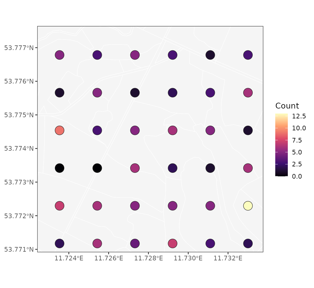
In the run used for the figures below, the simulation produced a total count of 147 over 36 plot observations, with a mean count of 4.08.
The plot counts are sparse relative to the fine raster domain. The fitted surface must borrow information through the covariate, the support model, and the spatial process.
Fit the count model
The fixed-size count model uses family = "negative_binomial" and requires size. The offset can be supplied as a numeric vector or as a column name in prep$B_sf. The Gaussian fit’s nugget variance is not part of this likelihood.
Code
prep <- cos_prepare(
  X_rast = X_rast,
  B_sf = B_sf,
  response_col = "y_nb",
  gamma = truth$gamma,
  taper_code = truth$taper_code,
  spatial = TRUE,
  n_threads = 2,
  missing = "renormalize",
  verbose = FALSE
)

priors <- cos_default_priors(
  prep = prep,
  beta_mu = c(intercept = 0, chm_z = 0),
  beta_sd = c(intercept = 2, chm_z = 1),
  sigma_shape = 2,
  sigma_scale = 1,
  phi_lower = 3 / 700,
  phi_upper = 3 / 40
)

fit <- cos_fit(
  prep = prep,
  priors = priors,
  family = "negative_binomial",
  size = size_true,
  offset = "log_exposure",
  n_chains = 1,
  starting = data.frame(sigma_sq = 0.60, phi = 3 / 250),
  tuning = c(log_sigma_sq = 0.25, z_phi = 0.25),
  n_batch = 25,
  batch_length = 5,
  seed = 1,
  n_threads = 2,
  verbose = FALSE
)

summary(fit)
For negative-binomial fits, cos_recover_B() selects the saved in-chain beta, omega_B, and eta_B draws. It does not run the Gaussian conjugate recovery step.
Code
rec <- cos_recover_B(
  fit = fit,
  burn_in = 35,
  thin = 4,
  n_samples = 12,
  seed = 1,
  n_threads = 2,
  verbose = FALSE
)
Fine-grid mean-count summaries
For a fine grid cell a, the conditional spatial mean and marginal variance are
E(\omega_a \mid \omega_B) = C_{aB} C_B^{-1}\omega_B,
\qquad
\mathrm{Var}(\omega_a \mid \omega_B) =
\sigma^2\{1 - C_{aB} C_B^{-1} C_{Ba}\}.
For each retained posterior draw and prediction cell, the package draws \omega_a from this one-dimensional normal conditional distribution, forms \eta_a = o_a + x_a^\top\beta + \omega_a, transforms with exp(), and summarizes the resulting mean-count draws. No joint fine-grid covariance matrix is formed.
Here offset_pred = 0, so the fine-grid map is a unit-exposure mean count surface. If the scientific target is a count for a particular pixel area, sample duration, or effort, use the corresponding log exposure in offset_pred.
Code
pred_cell <- which(stats::complete.cases(raster::getValues(X_rast)))
pred_coords <- raster::xyFromCell(X_rast[[1]], pred_cell)
X_pred <- as.matrix(raster::extract(X_rast, pred_cell))
colnames(X_pred) <- names(X_rast)

pred_fine <- cos_predict_fine(
  fit = fit,
  rec_B = rec,
  pred_coords = pred_coords,
  X_pred = X_pred,
  offset_pred = 0,
  spatial_uncertainty = "marginal",
  target = "latent",
  keep_samples = FALSE,
  verbose = FALSE
)
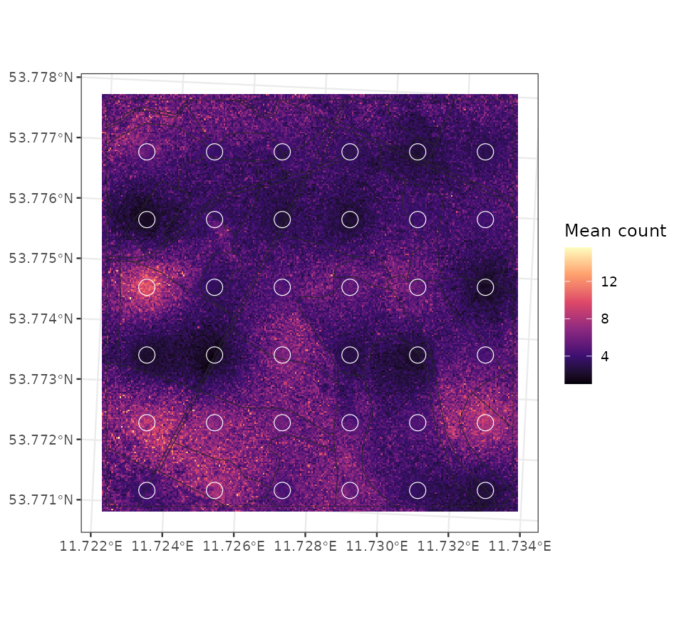
The fitted unit-exposure mean-count surface from the example run is:
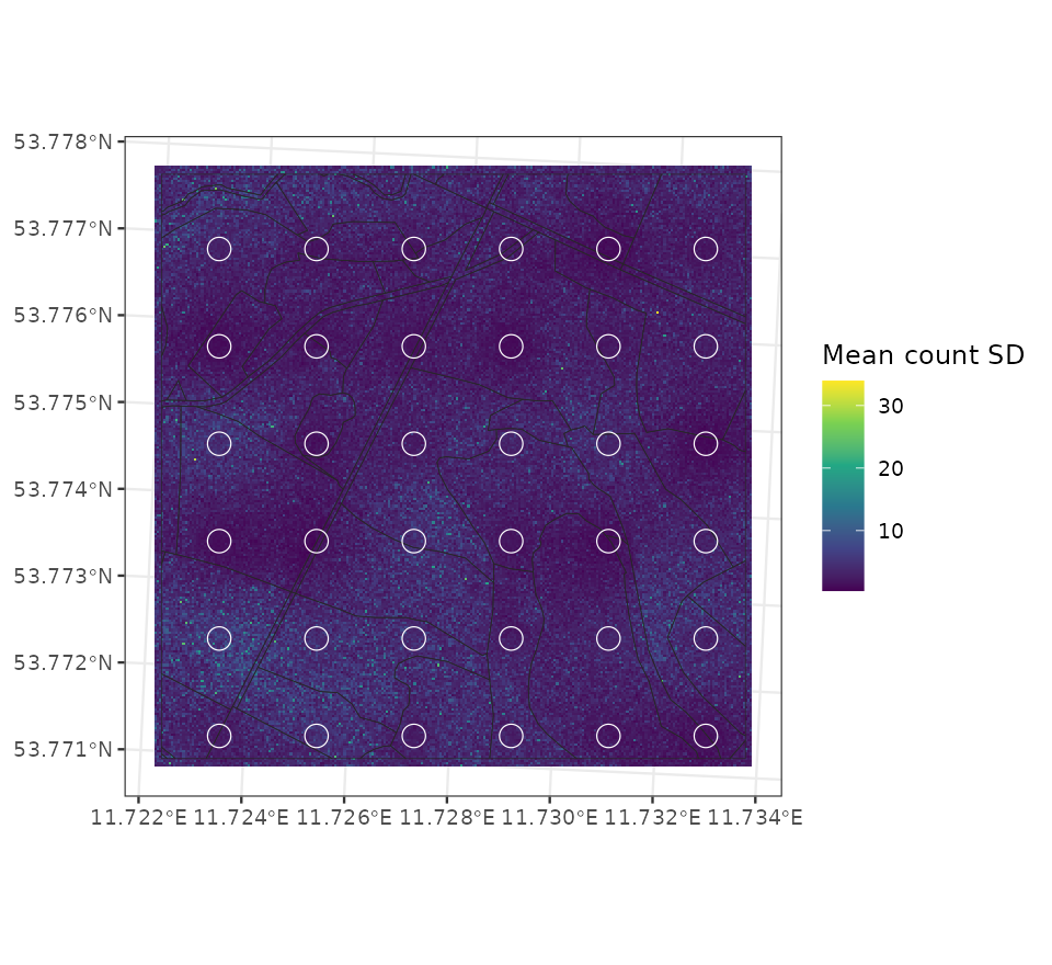
The next figure shows posterior standard deviations for the marginal mean-count summaries. These are independent marginal summaries by cell, not a joint simulated surface. Set keep_samples = TRUE to also retain draws and obtain posterior quantiles for intervals.
The distance summary from the same run was:
#>   mean_distance_to_plot_m mean_count_sd eta_sd
#> 1                   19.69         2.858  0.628
#> 2                   36.01         3.272  0.687
#> 3                   46.77         3.450  0.710
#> 4                   55.63         3.538  0.724
#> 5                   63.89         3.604  0.734
#> 6                   82.28         3.871  0.760
The posterior SD of the mean count increases with distance from the nearest observed plot, which is the expected behavior for marginal spatial prediction. The full mean-count uncertainty also includes fixed-effect and covariance-parameter uncertainty.
Areal count summaries
Fine-grid maps are useful diagnostics, but count summaries are often needed for stands or other areal units. cos_make_areal_blocks() builds the support weights, and cos_predict_areal() returns link-scale and mean-count summaries for each polygon.
In this example, the areal offset is the log of polygon area divided by the mean observed plot area. This makes the areal predictions expected counts for each polygon under an area-based exposure convention. For a real analysis, the offset should represent the exposure or sampling effort that defines the count target.
Code
U_sf <- st_read(
  system.file("extdata", "example_U.gpkg", package = "cosTapered"),
  quiet = TRUE
)

U_blocks <- cos_make_areal_blocks(
  U_sf = U_sf,
  X_rast = X_rast,
  id_col = "U_id",
  missing = "renormalize",
  verbose = FALSE
)

B_area_mean <- mean(as.numeric(st_area(B_sf)))
U_blocks$U_sf$log_exposure <- log(as.numeric(st_area(U_blocks$U_sf)) / B_area_mean)

pred_areal <- cos_predict_areal(
  fit = fit,
  rec_B = rec,
  U_blocks = U_blocks,
  offset_U = "log_exposure",
  spatial_uncertainty = "marginal",
  target = "latent",
  keep_samples = FALSE,
  verbose = FALSE
)
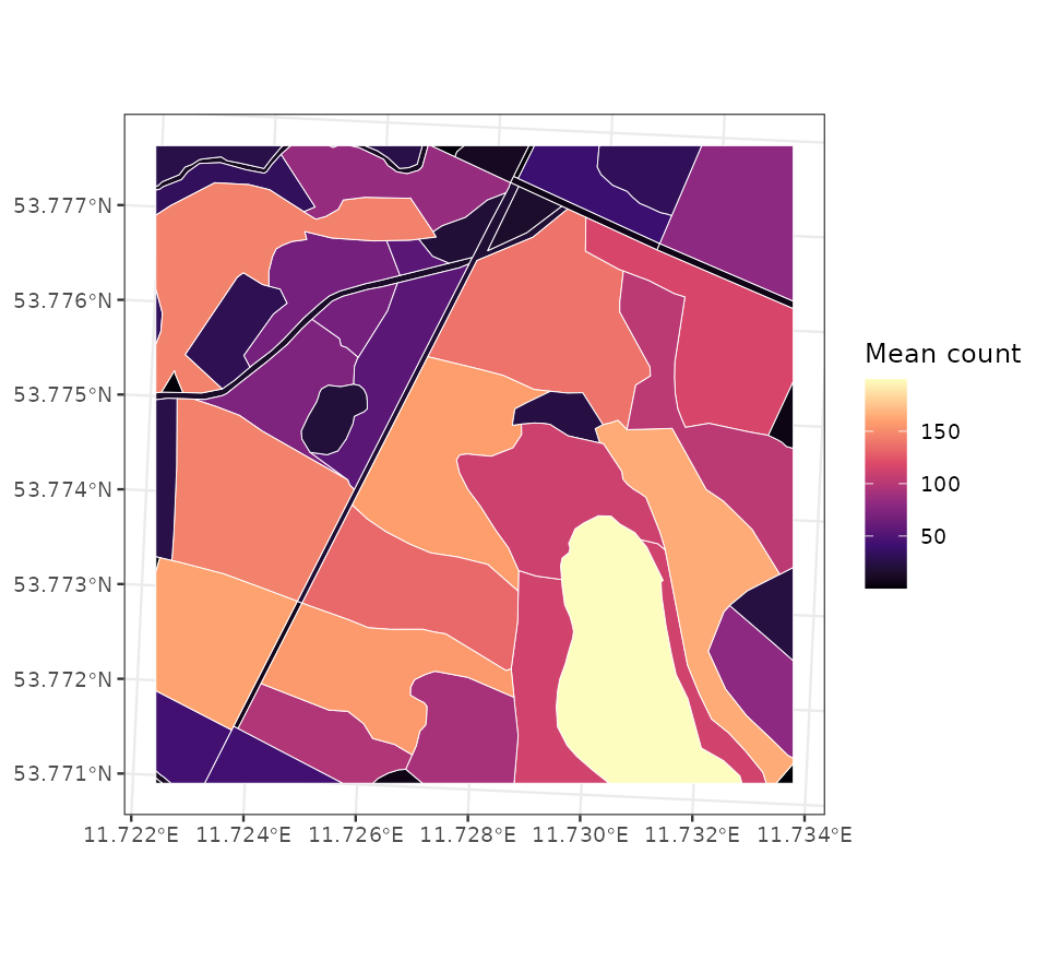
The areal posterior mean counts are:
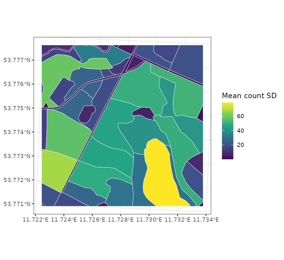
The areal posterior mean-count standard deviations are:
Use target = "latent" when the target is the expected count \mu_U. Use target = "observed" when the target is a future or replicated count observation on the same support and exposure. The observed target adds negative-binomial sampling variation around the latent mean.
Code
pred_areal_observed <- cos_predict_areal(
  fit = fit,
  rec_B = rec,
  U_blocks = U_blocks,
  offset_U = "log_exposure",
  spatial_uncertainty = "marginal",
  target = "observed",
  keep_samples = TRUE,
  verbose = FALSE
)

head(pred_areal_observed$summary)
For inference on individual stands, the marginal areal summaries are usually the relevant output. If stands will be combined into a larger reporting unit, predict directly for that dissolved reporting unit so the support and offset match the estimand.
The code above reproduces the simulation, fit, and prediction workflow. The original figure-generation script is not included in the public package.