This vignette illustrates the experimental binomial response model in cosTapered. The Gaussian COS model remains the default. The binomial path uses Polya-Gamma augmentation and keeps beta and the observed-support spatial effect omega_B explicit in the sampler state.
The example uses the package’s bundled raster covariate and plot polygons. We simulate binary plot outcomes from a weak fine-support covariate effect and a stronger spatial Gaussian process, fit the binomial COS model, and summarize predicted response probability over the fine grid.
The simulation, fitting, and prediction chunks are displayed without execution so that vignette builds stay quick. Run them in order to reproduce the model workflow. The figures and distance summaries are saved from an earlier example run; they are not regenerated during a vignette build. The short chain and 12 retained draws demonstrate the API; use longer chains, more draws, and convergence diagnostics for inference.
Model
For observed support B_l, the first binomial implementation uses
z_l \mid \eta_l, m_l
\sim \mathrm{Binomial}\{m_l, \mathrm{logit}^{-1}(\eta_l)\},
\qquad
\eta_l = \mathbf{x}_B(B_l)^\top \beta + \omega_B(B_l),
where z_l is the number of successes out of m_l trials and \mathbf{x}_B(B_l)^\top is row l of the observed-support design matrix X_B = H_{BA}X from cos_prepare(). The spatial effect \omega_B has the same tapered observed-support Gaussian process prior used by the Gaussian COS model. Conditional on Polya-Gamma weights, the sampler works with a Gaussian working response.
This model is on the observed support. It is not the same as averaging fine-support probabilities over a polygon. That distinction matters for interpretation and will remain explicit as response models are extended.
Simulate binary plot data
The code below constructs the raster design matrix, prepares the observed support, and simulates binary plot values. The covariate coefficient is small so the fine-support covariate explains little of the binary response variation. Most spatial pattern comes from the Gaussian process.
Code
library(cosTapered)
library(sf)
library(raster)

set.seed(1)

chm <- raster(system.file("extdata", "example_chm.tif", package = "cosTapered"))
names(chm) <- "chm"

chm_vals <- getValues(chm)
chm_center <- mean(chm_vals, na.rm = TRUE)
chm_scale <- sd(chm_vals, na.rm = TRUE)

chm_z <- chm
chm_z[] <- (chm_vals - chm_center) / chm_scale
names(chm_z) <- "chm_z"

intercept <- chm
intercept[] <- ifelse(is.na(chm_vals), NA_real_, 1)
names(intercept) <- "intercept"

X_rast <- stack(intercept, chm_z)
names(X_rast) <- c("intercept", "chm_z")

B_sf <- st_read(
  system.file("extdata", "example_B.gpkg", package = "cosTapered"),
  quiet = TRUE
)
truth <- readRDS(system.file("extdata", "example_truth.rds", package = "cosTapered"))

prep0 <- cos_prepare(
  X_rast = X_rast,
  B_sf = B_sf,
  response_col = "y_B",
  gamma = truth$gamma,
  taper_code = truth$taper_code,
  spatial = TRUE,
  n_threads = 2,
  missing = "renormalize",
  verbose = FALSE
)

beta_true <- c(intercept = -0.25, chm_z = 0.25)
sigma_sq_true <- 1
eff_range_true <- 250
phi_true <- 3 / eff_range_true

C_B_true <- cosTapered:::make_C_B_tapered_from_pairs_Rcall(
  C_B_pairs = prep0$C_B_pairs,
  phi = phi_true,
  n_threads = 2
)

R_C_true <- chol(C_B_true)
omega_B_true <- as.numeric(sqrt(sigma_sq_true) * t(R_C_true) %*% rnorm(nrow(prep0$X_B)))
eta_B_true <- as.numeric(prep0$X_B %*% beta_true + omega_B_true)
p_B_true <- plogis(eta_B_true)

B_sf$trials <- 1L
B_sf$y_bin <- rbinom(nrow(B_sf), size = 1L, prob = p_B_true)
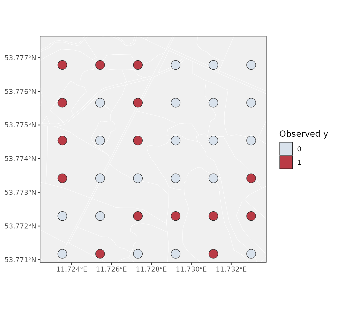
In the run used for the figures below, the simulation produced 15 successes among 36 binary plot observations.
The simulated zero/one responses are observed on plot polygons. The map below is useful as a first diagnostic: the observations are sparse and binary, so the fitted probability surface must borrow information through both the covariate and the spatial process.
Fit the binomial COS model
The binomial fit uses family = "binomial" and a trials vector or column name. The Gaussian fit’s nugget variance is not part of this likelihood.
Code
prep <- cos_prepare(
  X_rast = X_rast,
  B_sf = B_sf,
  response_col = "y_bin",
  gamma = truth$gamma,
  taper_code = truth$taper_code,
  spatial = TRUE,
  n_threads = 2,
  missing = "renormalize",
  verbose = FALSE
)

priors <- cos_default_priors(
  prep = prep,
  beta_mu = c(intercept = 0, chm_z = 0),
  beta_sd = c(intercept = 2, chm_z = 1),
  sigma_shape = 2,
  sigma_scale = 1,
  phi_lower = 3 / 700,
  phi_upper = 3 / 40
)

fit <- cos_fit(
  prep = prep,
  priors = priors,
  family = "binomial",
  trials = "trials",
  n_chains = 1,
  starting = data.frame(sigma_sq = 1, phi = 3 / 250),
  tuning = c(log_sigma_sq = 0.25, z_phi = 0.25),
  n_batch = 25,
  batch_length = 5,
  seed = 1,
  n_threads = 2,
  verbose = FALSE
)

summary(fit)
For binomial fits, cos_recover_B() selects the saved in-chain beta, omega_B, and eta_B draws. It does not run the Gaussian conjugate recovery step.
Code
rec <- cos_recover_B(
  fit = fit,
  burn_in = 35,
  thin = 4,
  n_samples = 12,
  seed = 1,
  n_threads = 2,
  verbose = FALSE
)
Fine-grid probability summaries
The binomial prediction path reports link-scale summaries and response probability summaries. For a fine grid cell a, the conditional spatial mean and marginal variance are
E(\omega_a \mid \omega_B) = C_{aB} C_B^{-1}\omega_B,
\qquad
\mathrm{Var}(\omega_a \mid \omega_B) =
\sigma^2\{1 - C_{aB} C_B^{-1} C_{Ba}\}.
The package uses independent marginal Monte Carlo draws for the response probability. For each retained posterior draw and prediction cell, it draws \omega_a from the one-dimensional normal conditional distribution above, forms \eta_a = x_a^\top\beta + \omega_a, transforms with plogis(), and summarizes the resulting probability draws. No joint fine-grid covariance matrix is formed.
For display, the code below predicts the full non-missing native fine-support raster domain. In the bundled example this is the 3 m by 3 m grid, and the marginal C++ prediction backend avoids forming the dense joint fine-grid covariance matrix.
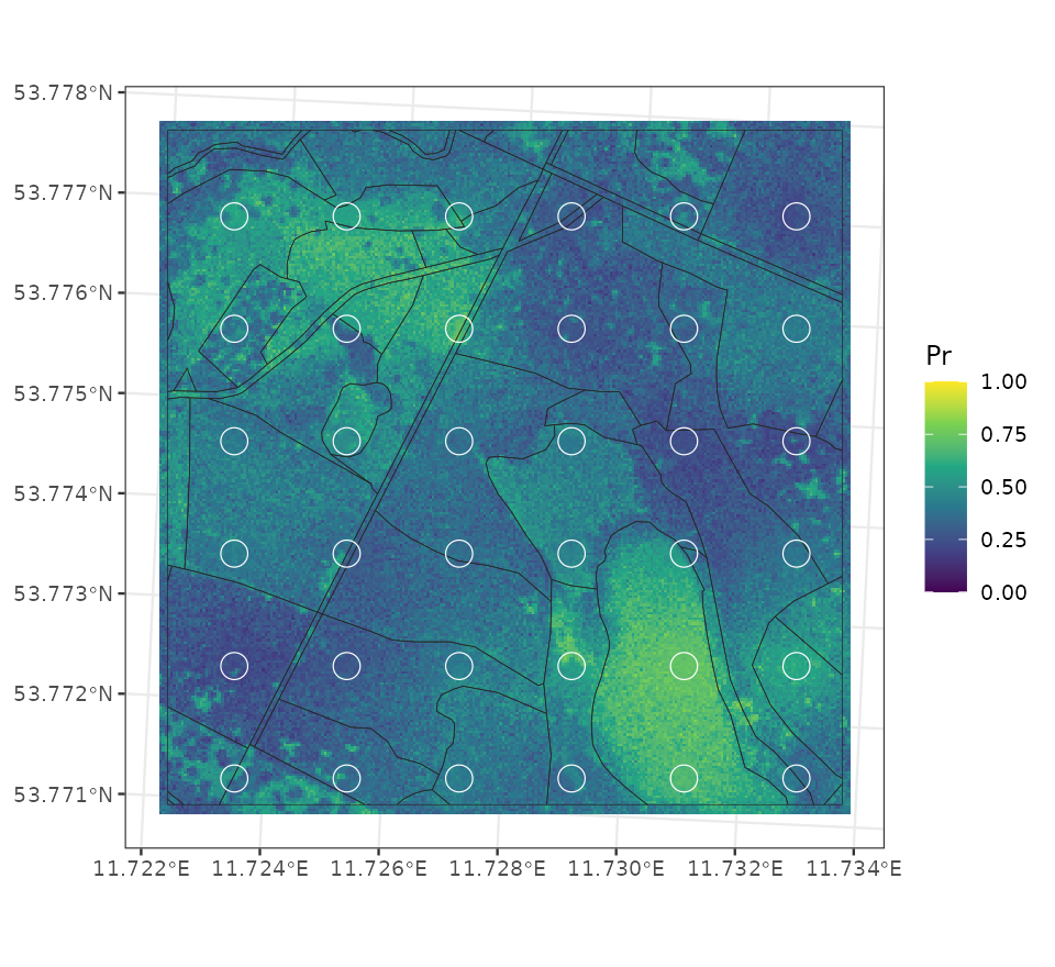
The fitted probability surface from the example run is:
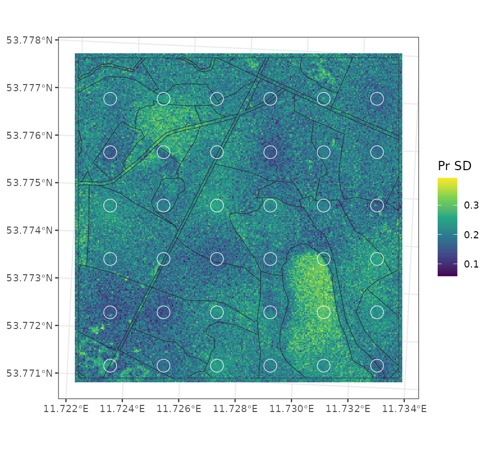
The next figure shows the posterior standard deviation of the marginal response probability. These are independent marginal summaries by cell, not a joint simulated surface.
The distance summary from the same run was:
  mean_distance_to_plot_m probability_sd
1                   19.69          0.205
2                   36.01          0.207
3                   46.77          0.209
4                   55.63          0.211
5                   63.89          0.210
6                   82.28          0.211
The table shows a small overall increase, with a dip in the fifth group; it is not monotone. Nearby observations can reduce conditional spatial uncertainty, but distance to the nearest plot alone does not determine it. The total posterior probability SD also depends on the link transformation, fixed effects, covariance parameters, and Monte Carlo variability.
Areal probability summaries
Fine-grid maps are useful for diagnostics, but management summaries are often needed on areal supports. The package uses the same marginal prediction logic for areal units. cos_make_areal_blocks() builds the support weights, and cos_predict_areal() returns link-scale and response-probability summaries for each polygon. For each draw, the areal probability is the inverse logit of the support-averaged linear predictor. It is not the area-weighted average of fine-cell probabilities. These are marginal summaries for separate units; the draws do not support joint comparisons across polygons. Use keep_samples = TRUE to obtain probability quantiles as well as means and SDs.
Code
U_sf <- st_read(
  system.file("extdata", "example_U.gpkg", package = "cosTapered"),
  quiet = TRUE
)

U_blocks <- cos_make_areal_blocks(
  U_sf = U_sf,
  X_rast = X_rast,
  id_col = "U_id",
  missing = "renormalize",
  verbose = FALSE
)

pred_areal <- cos_predict_areal(
  fit = fit,
  rec_B = rec,
  U_blocks = U_blocks,
  spatial_uncertainty = "marginal",
  keep_samples = FALSE,
  verbose = FALSE
)
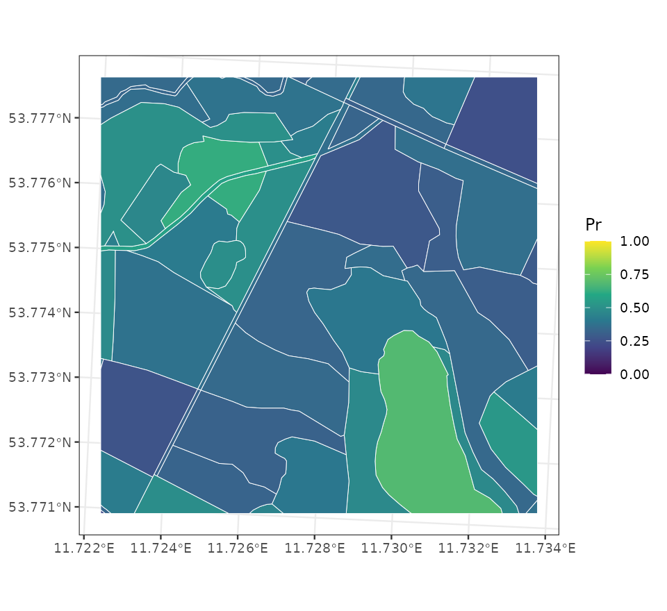
The areal posterior mean probabilities are:
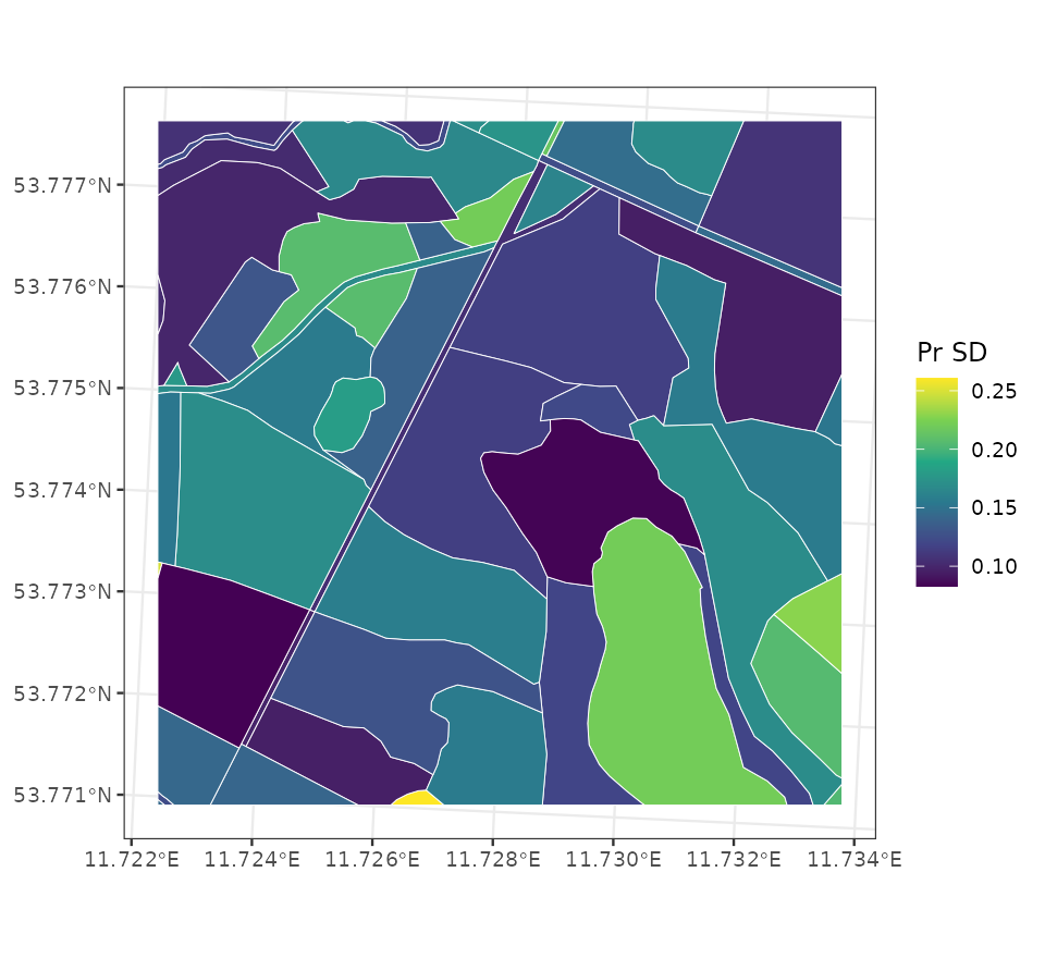
The areal posterior probability standard deviations are:
The code above reproduces the simulation, fit, and prediction workflow. The original figure-generation script is not included in the public package.