
Getting Started with cosTapered
Gaussian change-of-support fitting, fine-grid prediction, and areal summaries
Source:vignettes/cosTapered-introduction.qmd
1 Overview
cosTapered fits Bayesian change-of-support (COS) models for spatial data whose responses, covariates, and prediction targets are measured on different supports. In the COS setting considered here, covariates are represented on a fine raster grid, responses are observed on polygons, and predictions can be made for either fine raster cells or other polygon supports.
The fitting and prediction chunks below are displayed without execution to keep vignette builds quick. Run them in order for the complete workflow; the short chains illustrate the API and require longer runs and convergence diagnostics for inference.
Development of the package was motivated by data structures common in natural resource and forest inventory applications, where field responses are measured on plots, remotely sensed covariates are available as raster layers, and management decisions often require predictions for stands or other irregular areal units. The model follows the tapered COS formulation used by Zhang et al. (2024) for incompatible spatial forest damage data.
The main workflow is:
- Supply the raster covariate stack used to form the design matrix.
- Prepare observed-support weights with
cos_prepare(). - Specify priors with
cos_default_priors(). - Fit covariance parameters with
cos_fit(). - Recover observed-support latent quantities with
cos_recover_B(). - Predict fine-support or areal-support quantities with
cos_predict_fine()andcos_predict_areal().
The workflow keeps data preparation choices explicit. The raster stack defines the design matrix, including any intercept or transformed covariates; observed supports are supplied as polygons; the taper distance gamma is chosen before fitting; and areal predictions are returned as support averages, leaving any conversion to totals to the analysis context.
2 Example data
The package includes a small simulated example with a canopy-height raster, observed plot polygons, areal prediction polygons, a forest boundary, and known simulation truth.
Code
chm <- raster(system.file("extdata", "example_chm.tif", package = "cosTapered"))
names(chm) <- "chm"

B_sf <- st_read(system.file("extdata", "example_B.gpkg",
                            package = "cosTapered"), quiet = TRUE)
U_sf <- st_read(system.file("extdata", "example_U.gpkg",
                            package = "cosTapered"), quiet = TRUE)
forest_sf <- st_read(system.file("extdata", "example_forest.gpkg",
                                 package = "cosTapered"), quiet = TRUE)
truth <- readRDS(system.file("extdata", "example_truth.rds",
                             package = "cosTapered"))

truth[c("beta_true", "tau_B_sq_true", "sigma_sq_true",
        "eff_range_true", "phi_true", "gamma", "n_B", "n_U")]
#> $beta_true
#> intercept       chm
#>     45.00      1.25
#>
#> $tau_B_sq_true
#> [1] 8
#>
#> $sigma_sq_true
#> [1] 35
#>
#> $eff_range_true
#> [1] 250
#>
#> $phi_true
#> [1] 0.012
#>
#> $gamma
#> [1] 350
#>
#> $n_B
#> [1] 36
#>
#> $n_U
#> [1] 49
3 Supply the raster design
The model design matrix is taken from the layers in the raster stack. Here the stack contains an intercept layer and the canopy-height layer.
Code
chm_df <- as.data.frame(chm, xy = TRUE, na.rm = TRUE)
names(chm_df) <- c("x", "y", "chm")

ggplot() +
  geom_tile(data = chm_df, aes(x = x, y = y, fill = chm),
            width = xres(chm), height = yres(chm)) +
  geom_sf(data = U_sf, fill = NA, color = "white", linewidth = 0.25) +
  geom_sf(data = forest_sf, fill = NA, color = "black", linewidth = 0.55) +
  geom_sf(data = B_sf, fill = NA, color = "#c1121f", linewidth = 0.45) +
  scale_fill_viridis_c(option = "cividis") +
  coord_sf(expand = FALSE) +
  labs(title = "Raster covariate, observed plots, and prediction polygons",
       fill = "CHM", x = NULL, y = NULL) +
  theme_bw()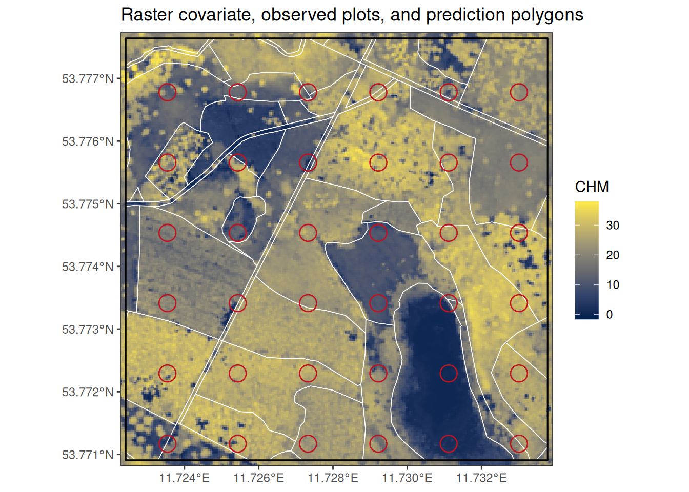
The observed plot responses are measured on the plot polygons. The COS model connects these plot-support responses to the raster covariates through support averaging.
Code
ggplot() +
  geom_sf(data = forest_sf, fill = "grey95", color = "grey40", linewidth = 0.3) +
  geom_sf(data = U_sf, fill = NA, color = "white", linewidth = 0.25) +
  geom_sf(data = B_sf, aes(fill = y_B), color = "grey15", linewidth = 0.25) +
  scale_fill_viridis_c(option = "magma") +
  coord_sf(expand = FALSE) +
  labs(title = "Observed Gaussian plot-support responses",
       fill = "y_B", x = NULL, y = NULL) +
  theme_bw()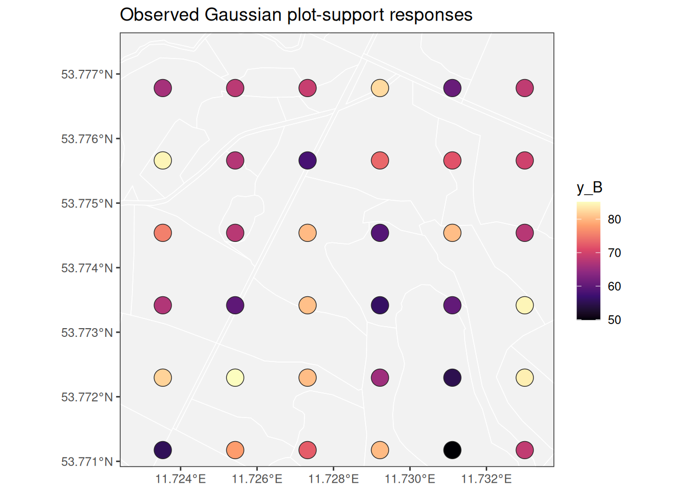
4 Prepare observed supports
cos_prepare() computes area weights linking observed polygons to raster cells, observed-support covariates, the observed-support nugget matrix, and the distance/taper information needed for spatial fitting.
This is the first model-building step after the raster design and observed polygons have been assembled.
By default, cos_prepare() stops if incomplete raster covariate cells would leave an observed-support row sum materially below one. This protects the support-average target. Use missing = "drop" or missing = "renormalize" only when the intended analysis should use covered cells rather than the full observed support.
Code
prep <- cos_prepare(
  X_rast = X_rast,
  B_sf = B_sf,
  response_col = "y_B",
  gamma = truth$gamma,
  taper_code = truth$taper_code,
  n_threads = 1,
  verbose = FALSE
)

summary(prep)
5 Specify priors
Priors are specified on the covariate scale supplied by the user. The package uses tau_B_sq, the average observed-support nugget variance, because this is usually easier to think about than the fine-support nugget variance tau_sq.
Code
priors <- cos_default_priors(
  prep = prep,
  beta_mu = c(intercept = 40, chm = 1),
  beta_sd = c(intercept = 20, chm = 2),
  tau_B_shape = 2,
  tau_B_scale = truth$tau_B_sq_true,
  sigma_shape = 2,
  sigma_scale = truth$sigma_sq_true,
  phi_lower = 3 / 600,
  phi_upper = 3 / 80
)
The exponential effective range is approximately 3 / phi. Thus phi_lower = 3 / 600 and phi_upper = 3 / 80 allow effective ranges from about 80 to 600 map units.
6 Fit the model
cos_fit() samples the collapsed posterior for covariance parameters. Use longer chains and multiple starting values for real analyses. burn_in is the first retained iteration in each chain, not a number of batches; burn_in = 50 below retains iteration 50 onward.
Code
fit <- cos_fit(
  prep = prep,
  priors = priors,
  n_chains = 3,
  starting = data.frame(
    tau_B_sq = truth$tau_B_sq_true * c(0.5, 1, 2),
    sigma_sq = truth$sigma_sq_true * c(0.5, 1, 2),
    phi = truth$phi_true * c(0.75, 1, 1.25)
  ),
  tuning = c(log_tau_B_sq = 0.25, log_sigma_sq = 0.25, z_phi = 0.25),
  n_batch = 100,
  batch_length = 25,
  seed = 1,
  verbose = TRUE
)

summary(fit, burn_in = 50)
plot(fit, burn_in = 50)
Trace plots should move across stable regions after burn-in. If phi piles up against a prior bound, revisit the effective range bounds or the taper distance gamma.
7 Recover observed-support quantities
cos_recover_B() samples regression coefficients, observed-support spatial effects, and observed-support latent means conditional on retained covariance parameter draws.
Code
rec_B <- cos_recover_B(
  fit = fit,
  burn_in = 50,
  n_samples = 100,
  seed = 1,
  verbose = FALSE
)

summary(rec_B, include_eta_B = TRUE)
8 Predict the fine grid
Fine-support prediction returns the latent raster-scale response by default. If pred_coords and X_pred are omitted, cos_predict_fine() predicts only on the complete raster cells intersecting the observed polygons, stored by cos_prepare(). To map the full raster domain, explicitly supply every complete cell as below. The example uses the native 3 m by 3 m grid.
For routine pixel-wise maps with uncertainty, use spatial_uncertainty = "marginal". This uses the faster marginal prediction backend: each fine cell receives its own one-dimensional conditional Gaussian draw for each retained posterior sample, without forming a dense joint covariance matrix across all cells. The resulting cell means, posterior standard deviations, and intervals are appropriate when cells are interpreted one at a time. Use spatial_uncertainty = "joint" only when a downstream summary combines cells and requires cross-cell covariance.
Code
pred_cell <- which(complete.cases(getValues(X_rast)))
pred_coords <- xyFromCell(X_rast[[1]], pred_cell)
X_pred <- as.matrix(extract(X_rast, pred_cell))
colnames(X_pred) <- names(X_rast)

pred_fine <- cos_predict_fine(
  fit = fit,
  rec_B = rec_B,
  pred_coords = pred_coords,
  X_pred = X_pred,
  spatial_uncertainty = "marginal",
  keep_samples = FALSE,
  n_threads = 2,
  verbose = FALSE
)

summary(pred_fine)
pred_fine$summary contains one row per predicted fine cell, including the cell coordinates, posterior mean, and posterior standard deviation. summary(pred_fine) summarizes those results across cells. Set keep_samples = TRUE to retain draws and add the 2.5%, 50%, and 97.5% posterior quantiles; interval summaries are not returned with keep_samples = FALSE. The same rule applies to areal predictions.
9 Predict areal supports
Areal prediction first builds prediction-support blocks and then predicts support averages. cos_make_areal_blocks() uses the same missing-covariate policy as cos_prepare(). For per-stand or per-polygon estimates with valid one-unit-at-a-time uncertainty, use spatial_uncertainty = "marginal".
Code
U_blocks <- cos_make_areal_blocks(
  U_sf = U_sf,
  X_rast = X_rast,
  id_col = "U_id",
  verbose = FALSE
)

pred_U <- cos_predict_areal(
  fit = fit,
  rec_B = rec_B,
  U_blocks = U_blocks,
  spatial_uncertainty = "marginal",
  keep_samples = FALSE,
  n_threads = 2,
  verbose = TRUE
)

summary(pred_U)
Prediction functions default to target = "latent". Use target = "observed" when the prediction should include support-level nugget variation on the requested support. For areal prediction, spatial_uncertainty = "marginal" returns marginal samples for each prediction unit, not joint samples across units; do not use those samples for totals, contrasts, or rankings that require cross-unit covariance.
10 Cross validation
cos_cv_observed() performs K-fold cross validation by refitting the model to training plots and predicting held-out plot polygons. By default it scores the observed response. In simulations with known latent truth, it can score both latent and observed targets from the same refits.
Code
set.seed(1)
fold_id <- sample(rep(seq_len(10), length.out = nrow(B_sf)))

cv <- cos_cv_observed(
  fit = fit,
  X_rast = X_rast,
  B_sf = B_sf,
  target = c("latent", "observed"),
  latent_col = "eta_B_true",
  k = 10,
  fold_id = fold_id,
  fit_args = list(n_batch = 50, batch_length = 8),
  recover_args = list(burn_in = 100, n_samples = 60),
  seed = 1,
  verbose = FALSE
)

summary(cv)
For model-comparison guidance, see the spatial-guidance vignette. For model and computational details, see the model-details vignette.
11 Reference
Zhang, L., Finley, A. O., Nothdurft, A., and Banerjee, S. (2024). Bayesian modeling of incompatible spatial data: A case study involving Post-Adrian storm forest damage assessment. International Journal of Applied Earth Observation and Geoinformation, 135, 104224. https://doi.org/10.1016/j.jag.2024.104224