Tapered Change-of-Support Spatial Response Models • cosTapered

cosTapered implements and expands on the Bayesian change-of-support methods of Zhang et al. (2024) for forest inventory and remote-sensing problems where responses, predictors, and prediction targets live on different spatial supports.

Visit the cosTapered documentation website for getting-started guides, vignettes, and the function reference.

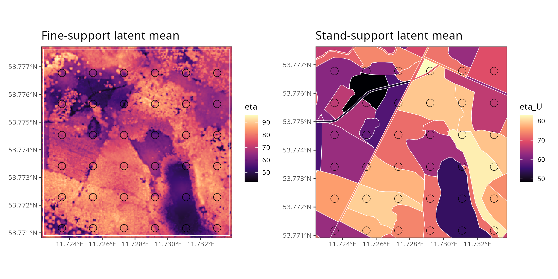
The motivating case is common in forest applications: LiDAR-derived predictors are available on a fine raster grid, field responses are observed on larger fixed-area plots, and final summaries are needed for irregular stands or other management units. Rather than forcing everything onto one arbitrary support before modeling, cosTapered defines a latent response surface on the fine predictor grid and links plots and stands to that surface through area-weighted averages.

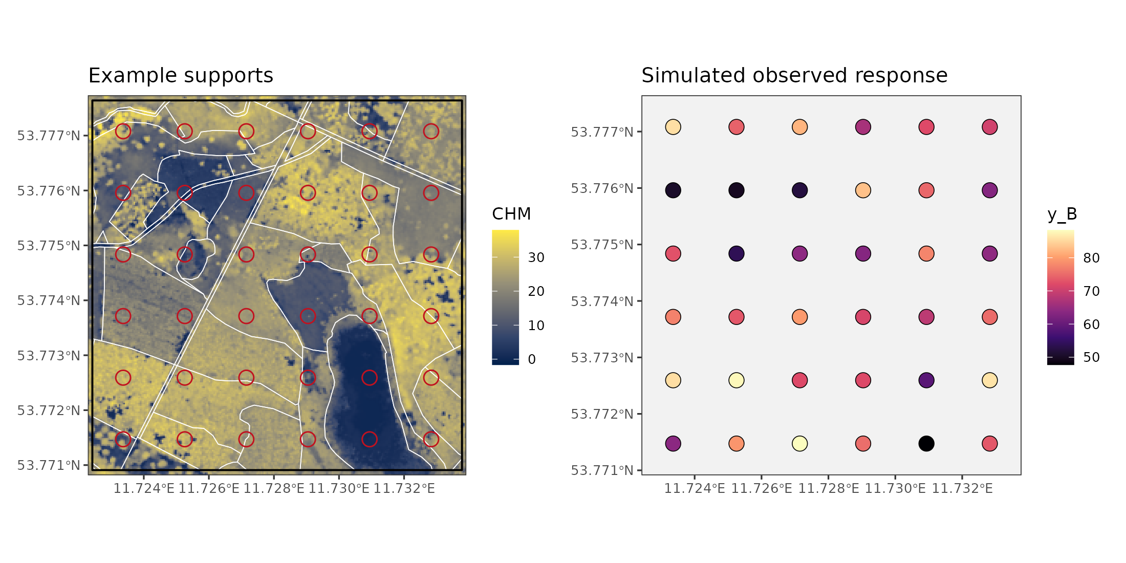
Example CHM raster, stand polygons, observed plots, and simulated plot response

Plots and stands are treated symmetrically: both are averages of the same fine-support latent process over their footprints. The main Gaussian response model uses a tapered exponential covariance for spatial residual variation so that large raster and polygon-support problems remain computationally manageable. Experimental binomial logit and fixed-size negative-binomial response paths are also available for observed-support binary, binomial, and count responses.

Example fine-support and stand-support latent predictions

Features

Prepare raster covariates and observed-support polygons with cos_prepare().
Fit Gaussian, experimental binomial, or fixed-size negative-binomial change-of-support models with cos_fit().
Recover observed-support latent quantities with cos_recover_B().
Predict fine-support or areal-support targets with cos_predict_fine() and cos_predict_areal().
Choose latent or observed prediction targets, where supported, with target = "latent" or target = "observed".
Choose how unobserved spatial prediction uncertainty is handled with spatial_uncertainty = "conditional_mean", "marginal", or "joint" where supported by the response family.
Run Gaussian observed-support K-fold validation with cos_cv_observed().

Installation

cosTapered requires R 4.1 or later. The main package dependencies are installed by remotes::install_github(), including sf, raster, exactextractr, Matrix, and BayesLogit. BayesLogit is required because the experimental binomial and negative-binomial response samplers use Polya-Gamma random variates through its C/C++ interface. exactextractr is required to compute the exact fraction of each raster cell covered by plot and areal prediction polygons, which defines the change-of-support averaging weights used by the model.

On Linux, sf and exactextractr may also require geospatial system libraries such as GDAL, GEOS, PROJ, and udunits before their R packages can be compiled.

install.packages("remotes")
remotes::install_github("finleya/cosTapered", subdir = "cosTapered")

To build the package vignettes from source, install the suggested vignette tools and the Quarto command-line tool:

install.packages(c("ggplot2", "knitr", "quarto", "rmarkdown"))
remotes::install_github(
  "finleya/cosTapered",
  subdir = "cosTapered",
  build_vignettes = TRUE
)

Quarto itself must also be available on the system path; see https://quarto.org/docs/get-started/. The repository includes the model and software PDF; HTML vignettes are generated when you build them. The vignette() calls below require an installation with build_vignettes = TRUE.

The pkgdown site presents all five vignettes as articles, alongside the function reference.

Example

library(cosTapered)
library(raster)
library(sf)

chm <- raster(system.file("extdata", "example_chm.tif",
                          package = "cosTapered"))
names(chm) <- "chm"

B_sf <- st_read(system.file("extdata", "example_B.gpkg",
                            package = "cosTapered"), quiet = TRUE)

intercept <- chm
intercept[] <- ifelse(is.na(getValues(chm)), NA_real_, 1)
names(intercept) <- "intercept"

X_rast <- stack(intercept, chm)
names(X_rast) <- c("intercept", "chm")

prep <- cos_prepare(
  X_rast = X_rast,
  B_sf = B_sf,
  response_col = "y_B",
  gamma = 350,
  n_threads = 1,
  verbose = FALSE
)

summary(prep)

truth <- readRDS(system.file("extdata", "example_truth.rds",
                             package = "cosTapered"))

priors <- cos_default_priors(
  prep = prep,
  beta_mu = c(intercept = 40, chm = 1),
  beta_sd = c(intercept = 20, chm = 2),
  tau_B_shape = 2,
  tau_B_scale = truth$tau_B_sq_true,
  sigma_shape = 2,
  sigma_scale = truth$sigma_sq_true,
  phi_lower = 3 / 600,
  phi_upper = 3 / 80
)

fit <- cos_fit(
  prep = prep,
  priors = priors,
  n_chains = 1,
  starting = c(
    tau_B_sq = truth$tau_B_sq_true,
    sigma_sq = truth$sigma_sq_true,
    phi = truth$phi_true
  ),
  tuning = c(log_tau_B_sq = 0.25, log_sigma_sq = 0.25, z_phi = 0.25),
  n_batch = 50,
  batch_length = 10,
  seed = 1,
  verbose = FALSE
)

summary(fit, burn_in = 25)

This short chain demonstrates the API. Use longer chains and convergence diagnostics for inference. burn_in is the first retained iteration in each chain, so burn_in = 25 keeps iteration 25 onward.

See the introductory package vignette for a complete Gaussian workflow:

vignette("cosTapered-introduction", package = "cosTapered")

The package includes complementary documents for different levels of detail:

Getting started: basic Gaussian workflow.
Model and computing details: model parameterization, computation, support targets, and prediction uncertainty.
Spatial guidance: practical guidance on when spatial COS helps.
Binomial responses: experimental Polya-Gamma binomial response workflow.
Negative-binomial responses: experimental fixed-size negative-binomial count response workflow with offsets and areal count summaries.
Model and software PDF: model and software details with posterior calculations.

vignette("cosTapered-model", package = "cosTapered")
vignette("cosTapered-spatial-guidance", package = "cosTapered")
vignette("cosTapered-binomial", package = "cosTapered")
vignette("cosTapered-negative-binomial", package = "cosTapered")
system.file("doc", "cosTapered.pdf", package = "cosTapered")

Model Scope

The current package supports a tapered exponential covariance with Wendland or spherical compact tapers and a proper normal prior for regression coefficients. Users supply the raster design matrix they want the model to use; cosTapered does not automatically add intercepts, scale covariates, or buffer points.

Prediction functions distinguish the underlying support average from an observed-scale prediction. For Gaussian fits, use target = "latent" for the underlying mean response, denoted eta in the model, and target = "observed" when the prediction should include finite-cell or support-averaged nugget variation. Binomial prediction currently reports the latent link scale and response probability. Negative-binomial prediction uses target = "latent" for the expected count and target = "observed" for a future or replicated count draw.

The main prediction choices are:

Response family	Fine-support prediction	Areal prediction	Spatial uncertainty
Gaussian	Latent mean, or response with fine-cell nugget	Latent support average, or response with support-averaged nugget	`conditional_mean` or `marginal`; also `joint` for fine support
Binomial	Latent link and probability	Latent support-averaged link and its inverse-logit probability	`conditional_mean` or `marginal`
Negative-binomial	Latent link and expected count, or an observed count draw	Latent support-averaged link plus offset and expected count, or an observed count draw	`conditional_mean` or `marginal`

Both prediction functions default to spatial_uncertainty = "conditional_mean". Set spatial_uncertainty = "marginal" explicitly for marginal uncertainty. Posterior means and SDs are returned with keep_samples = FALSE; use keep_samples = TRUE to also obtain draws and 2.5%, 50%, and 97.5% quantiles.

Without pred_coords and X_pred, fine prediction covers only the complete raster cells intersecting observed polygons. Supply both arguments to map the full raster domain, as shown in the introductory article.

For Gaussian fine-support prediction, spatial_uncertainty = "joint" draws from the joint conditional Gaussian surface and can be expensive for large rasters. spatial_uncertainty = "marginal" draws independent marginal conditional values for each prediction cell or areal unit. Use the marginal option for per-cell, per-stand, or per-polygon posterior means, SDs, and intervals when units are interpreted separately. For areal prediction, samples are marginal by unit and should not be used for totals, contrasts, or rankings that require cross-unit covariance. spatial_uncertainty = "conditional_mean" is a plug-in fitted-surface summary and does not represent full prediction uncertainty.

The binomial and fixed-size negative-binomial response models use Polya-Gamma augmentation through BayesLogit. Binomial prediction reports link-scale summaries and response probability summaries. Negative-binomial prediction uses a fixed size parameter, supports offsets such as log exposure, reports link-scale and mean-count summaries with target = "latent", and can simulate observed count predictions with target = "observed". For these non-Gaussian models, aggregation occurs on the linear-predictor scale: areal probabilities are not averages of fine-cell probabilities, and areal expected counts are not sums of fine-cell expected counts. Prediction offsets must express the intended exposure and default to zero; fitted offsets are not automatically reused. The Polya-Gamma response paths support spatial_uncertainty = "conditional_mean" and "marginal"; they do not produce joint prediction surfaces.

Reference

Zhang, L., Finley, A. O., Nothdurft, A., and Banerjee, S. (2024). Bayesian modeling of incompatible spatial data: A case study involving Post-Adrian storm forest damage assessment. International Journal of Applied Earth Observation and Geoinformation, 135, 104224. https://doi.org/10.1016/j.jag.2024.104224