Adaptive Block Random-Walk Metropolis Sampler

Runs an adaptive block random-walk Metropolis sampler. This function is used internally by cos_fit and is exported for development and diagnostics.

Usage

lapMetropBlock(ltd, starting, tuning = NULL, batch = 100,
  batch.length = 50, accept.rate = 0.234, c0 = 1, c1 = 0.8,
  report = 10, verbose = TRUE)

Arguments

ltd

Function returning the log target density at a parameter vector.

starting

Named numeric vector of starting values.

tuning

Optional proposal scale vector.

batch

Number of adaptive batches.

batch.length

Number of iterations per batch.

accept.rate

Target acceptance rate.

c0, c1

Adaptation constants.

report

Batch reporting interval.

verbose

Logical; if TRUE, print sampler progress.

Value

A list containing transformed-parameter samples, log-posterior samples, acceptance indicators, batch acceptance rates, and final proposal covariance information.

Examples

set.seed(1)

# Target a correlated bivariate normal so the block sampler has something
# nontrivial to learn.
mu <- c(x = 0, y = 0)
Sigma <- matrix(c(1.0, 0.85,
                  0.85, 1.5), 2, 2,
                dimnames = list(names(mu), names(mu)))
Sigma_inv <- solve(Sigma)

ltd <- function(x) {
  z <- x - mu
  as.numeric(-0.5 * t(z) %*% Sigma_inv %*% z)
}

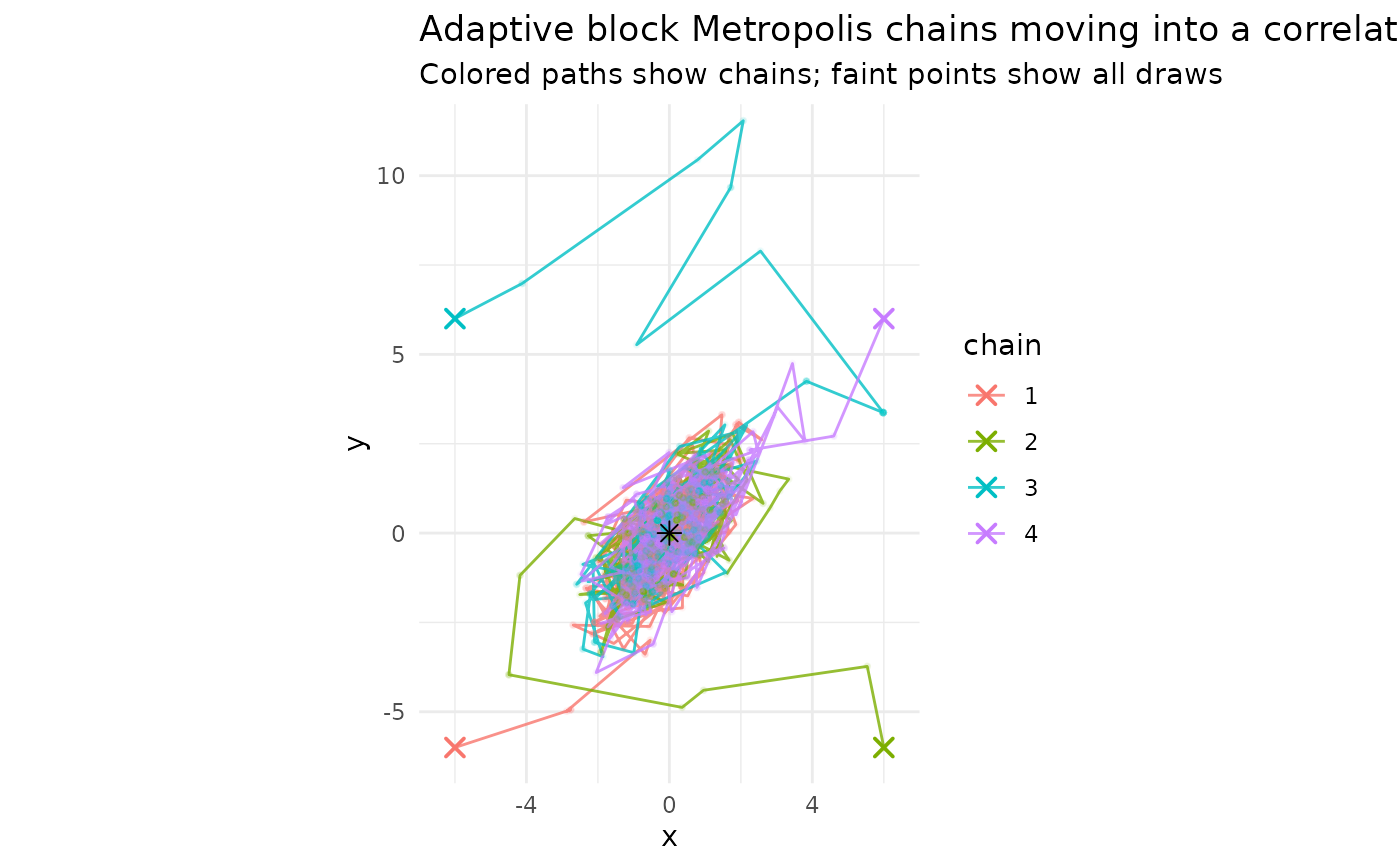
# Start four chains on opposite sides of the mode and let them move inward.
starts <- list(
  c(x = -6, y = -6),
  c(x = 6, y = -6),
  c(x = -6, y = 6),
  c(x = 6, y = 6)
)
start_df <- do.call(rbind, lapply(seq_along(starts), function(ch) {
  data.frame(chain = factor(ch), x = starts[[ch]][["x"]], y = starts[[ch]][["y"]])
}))

# Use a common proposal scale and run each chain separately.
fits <- lapply(starts, function(start) {
  lapMetropBlock(
    ltd,
    starting = start,
    tuning = c(x = 1.5, y = 1.5),
    batch = 30,
    batch.length = 20,
    verbose = FALSE
  )
})

# Combine draws so we can inspect the trajectories in one figure.
draws <- do.call(rbind, lapply(seq_along(fits), function(ch) {
  dat <- as.data.frame(fits[[ch]]$p.theta.samples)
  dat$chain <- factor(ch)
  dat$iter <- seq_len(nrow(dat))
  dat
}))
path_df <- do.call(rbind, lapply(seq_along(starts), function(ch) {
  rbind(
    data.frame(
      chain = factor(ch, levels = levels(draws$chain)),
      iter = 0L,
      x = starts[[ch]][["x"]],
      y = starts[[ch]][["y"]]
    ),
    draws[as.character(draws$chain) == as.character(ch), c("chain", "iter", "x", "y")]
  )
}))

# The paths should move in from the sides and the point cloud should fill in
# the target shape over time. Plotting requires the suggested ggplot2 package.
if (requireNamespace("ggplot2", quietly = TRUE)) {
  library(ggplot2)

  ggplot(draws, aes(x = x, y = y, group = chain, color = chain)) +
    geom_path(data = path_df, aes(x = x, y = y, group = chain, color = chain),
              linewidth = 0.5, alpha = 0.8) +
    geom_point(alpha = 0.05, size = 0.7) +
    geom_point(data = start_df, shape = 4, size = 2.5, stroke = 1) +
    geom_point(
      data = data.frame(x = mu["x"], y = mu["y"]),
      aes(x = x, y = y),
      inherit.aes = FALSE,
      shape = 8,
      size = 2.6,
      color = "black"
    ) +
    coord_equal(xlim = c(-7, 7), ylim = c(-7, 12), expand = FALSE) +
    labs(
      title = "Adaptive block Metropolis chains moving into a correlated target",
      subtitle = "Colored paths show chains; faint points show all draws",
      x = "x",
      y = "y",
      color = "chain"
    ) +
    theme_minimal(base_size = 11)
}